[
 Producing wound components]
[A guide to the terminology used in the science of magnetism]
[ Power loss in wound components]
[ Faraday's law]
Producing wound components]
[A guide to the terminology used in the science of magnetism]
[ Power loss in wound components]
[ Faraday's law]
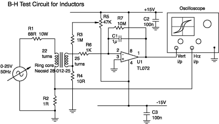
It works best with ring cores (toroids) but should be usable with other shapes having a closed magnetic path. The circuit, as shown, will plot the hysteresis loop for a half-inch diameter, high permeability ferrite ring; adaptations for other components are also given.
See also ...
[
Producing wound components]
[A guide to the terminology used in the science of magnetism]
[ Power loss in wound components]
[ Faraday's law]
(If the above image is broken then you need an updated browser: NS 4.4 or later)
Tolerances are only significant on R2, R6 and C1 (which is polyester
or polycarbonate). C2 and C3 are ceramic.
Winding the core
I chose to use two windings. Although a more complicated circuit could
be devised (which only required one winding) this circuit is cheaper,
easier to understand and more flexible. There is nothing special about
the number of turns used - just as long as you know how many you have.
The secondary can be made from wire that is as thin as you like, while the
primary need only be sufficiently thick not to get hot enough to heat the
core much (the saturation level falls fairly
rapidly with temperature). I used 0.2mm and 0.5mm respectively.
The equipment
You will need a source of AC current of about 0.3 amp.
If you're feeling lazy and don't want to wind as many turns on the
primary then you'll need a higher current. I used a lab supply, which
gave up to 25V at 50Hz, together with R1 to limit the current.
You can improvise other solutions. A mains variac followed by a step-down
transformer should work well.
Note: if you wish to measure very small rings with low permeability (such as those used in radio receivers) then you may need a source running at a few kilohertz in order to get sufficient secondary voltage. If you do this then you should also decrease C1.
The oscilloscope must be a dual channel model able to operate in an 'X-Y mode' (with the horizontal deflection controlled by a signal input rather than the timebase). I used an HP 54600 digital storage 'scope. A DSO is handy if you wish to plot initial magnetization curves.
Component tolerances for R2, R6 and C1
will affect the accuracy of your results.
Adjusting the circuit
The op-amp is used as a voltage integrator. A common problem
with this circuit is drift due to voltage and current offsets.
R7 helps keep drift under control but you will still need to
adjust R5 so that, with no signal in or out of the integrator,
the output on pin 1 remains steady.
Interpreting the curves
The following curve was obtained using a low current:
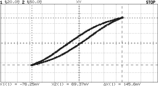
X-axis = voltage on R2. Y-axis = Vo (voltage on U1 pin 1)
This shows the characteristic hysteresis effect. Looking at the horizontal axis you see that the limits of the curve span a change in voltage of 146mV. Because R2 is 1 ohm you know that the primary current, Ip, changes by 146mA. From this you can find the change in field strength as:
H = Np×Ip / le Am-1
Where Np is the number of turns on the primary. For the core I used this gives H = 22×0.146/0.0276=116Am-1.
OK, that's the field strength found. flux density is a bit trickier. Faraday's Law tells us:
Vs = Ns×d/dt volts
Where Vs is the voltage on the secondary winding and
Ns is the number of turns on the secondary and is the the magnetic flux in the core. Now, all text books on
op-amps give the result:
dVo/dt = -Vs/(C1R6) volts
Where Vo is the voltage on pin 3. Substituting the previous result for Vs we get:
dVo/dt = -Ns(d
We have time rates of change on both sides of this equation so we can integrate wrt time and get:
Vo = -Ns
This is a good result because it establishes that the op-amp voltage is proportional to the core flux.
Putting in the known values:
We now get the flux density from:
B =The core has a roughly rectangular cross section of 6.3 × 3.2 = 20.2 mm2. So
B = 9.56e-6/20.2e-6 = 0.473 teslaNow we can work out the permeabilty (at this level of field strength) from:
µ = µ0 µr = B/H H m-1
4e-7µr = 0.473/116 H m-1
Giving µr = 3240.
Finding the hysteresis losses
Save the image above to disk and then open it with an image editing
program such as Photoshop.
Draw a rectangular selection marquee around
the limits of the curve and choose image:histogram. At the bottom of
the dialog box is a value for the total number of pixels selected:
45122. Now, using the polygon lasso tool trace the outline of the
hysteresis loop. This encloses 4605 pixels. If our loop had the
completely rectangular shape then the energy contained would be:
WR = H × B = 116 × 0.473 = 54.9 J m-3
However, the actual area of our loop is smaller by the fraction 4605/45122 giving an actual energy value of
WA = 54.9 × 4605/45122 = 5.60 J m-3
If we ran the core at 25 kHz this would mean a hysteresis loss rate of
P = 5.60 × 25e3 = 140 kW m-3
The mean core diameter is 9.5 mm so the volume is
VT = 20.2e-6 × 9.5e-3
So the total core hysteresis loss is
P = 140e3 × 6.03e-7 = 84.4 mW
Now, the above calculation isn't to be taken too seriously - there are several shaky assumptions, but as an indication then it should be worthwhile.
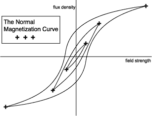
When the primary current is increased you will see a curve something like this:

X-axis = voltage on R2. Y-axis = voltage on U1 pin 1
Note the change of scale on the X-axis. The difference in shape is due to the onset of saturation.
If you repeat this measurement at different values of primary current then you can get a curve like this:
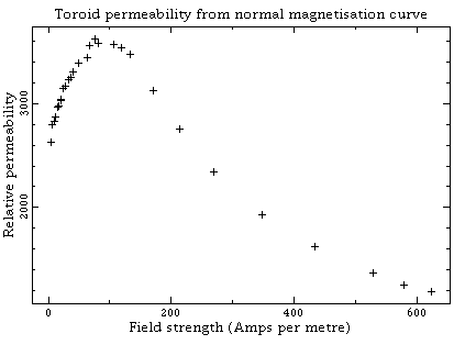
X-axis = Field strength (Am-1).
Y-axis = relative permeability
Incidentally, as you raise the primary current the tip of the hysteresis loop traces out a normal magnetization curve. It is similar in shape to the initial magnetization curve, and is a useful way of describing the material behavior.
Troubleshooting
If you have insufficient signal on the output of the integrator then
try reducing C1. You could also reduce R6 but
there's a risk that the secondary current will start to affect the H
field.