[
 The ESU Advisor Index]
[Producing wound components]
[A guide to the terminology used in the science of magnetism]
The ESU Advisor Index]
[Producing wound components]
[A guide to the terminology used in the science of magnetism]
Your life as a designer of transformers, for example, would be far simpler if you did not need to worry about power losses; you would simply select a part having the turns ratio needed - and that would be that. It's the requirements to keep the losses under control that largely determines whether your transformer weighs one gram and costs one dollar or weighs one ton and costs ten thousand dollars.
Power is lost in an inductor through several different mechanisms:
See also ...
[
The ESU Advisor Index]
[Producing wound components]
[A guide to the terminology used in the science of magnetism]
| Temperature (°C) | 20 | 40 | 60 | 80 | 100 |
|---|---|---|---|---|---|
| m (Mullard, 1979) | 1.0 | 1.079 | 1.157 | 1.236 | 1.314 |
You can conveniently estimate the resistance of a wire as
R = 0.022 / DW2 ohms per metrewhere DW is the diameter of the conductor in millimetres. Usually, you will know the length of a winding from
lw = Nwhere N is the number of turns and Dav is the average diameter of the winding in metres. Your copper losses will then beDav metres
PW = 0.022 × lw × (I / DW)2 watts
where I is the RMS current in the winding.
The usual range of current densities seen in power transformers lies between about 1.5 to 5 amps per square millimetre. Higher values lead to lower efficiency and a shorter life for the insulation. Lower values lead to size and initial cost problems. A good starting point is 3A millimetre-2. You can look up the diameter corresponding to this density in the table below. If efficiency is important then choose a lower current density. If size, cost or frequency range are important choose a high density.
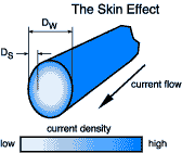
Unfortunately the above analysis holds only for low frequencies. Copper losses increase with frequency due to the skin effect.
Wire diameters are still often specified by British Standard Wire Gauge number.
| Standard Wire Gauge | Diam. milli- metres | Current at 3Amp mm-2 |
|---|---|---|
| 10 | 3.24 | 25 |
| 12 | 2.64 | 16 |
| 14 | 2.03 | 10 |
| 16 | 1.62 | 6 |
| 18 | 1.22 | 3.5 |
| 20 | 0.91 | 2 |
| 22 | 0.71 | 1.2 |
| 24 | 0.56 | 0.74 |
| 26 | 0.46 | 0.5 |
| 28 | 0.376 | 0.33 |
| 30 | 0.304 | 0.22 |
| 32 | 0.274 | 0.18 |
| 34 | 0.234 | 0.13 |
| 36 | 0.193 | 0.088 |
| 38 | 0.152 | 0.054 |
| 40 | 0.122 | 0.035 |
| 42 | 0.102 | 0.025 |
| 44 | 0.081 | 0.015
|
DS = 1.98 * sqr(R / (µ * f))

       where  R is resistance of 1cm^3
              DS is skin depth in inches
              f is frequency in hertz
              µ is the permeability of material in henrys per metre
| 50Hz | 1kHz | 100kHz | 1MHz | 10MHz | |
|---|---|---|---|---|---|
| Copper | 0.3 | 0.08 | 0.008 | 0.0025 | 0.0008 |
| Aluminium | 0.45 | 0.12 | 0.012 | 0.0035 | 0.0012 |
| Cold steel | 0.65 | 0.15 | 0.015 | 0.004 | 0.0015 |
| Graphite | 8.0 | 1.7 | 0.2 | 0.05 | 0.02
|
Skin effect occurs because current flow moves away from those regions of the conductor having the strongest magnetic field. A consequence of this is that the number of flux linkages between turns will be reduced. Therefore skin effect produces a decrease in inductance; of about 2%, though more if the wire is short.
Having chosen a diameter of wire that can cope with the current at zero Hz you should check that skin effect is not going to be a problem at the frequency at which you actually need to work. The formula below (Terman) gives the diameter of wire that will suffer a 10% increase in resistance at the frequency of operation, f (in Hz) -
DW = 200 / f0.5 millimetres
This formula applies for isolated conductors. In a coil surrounded by other turns the actual resistance will be higher because of the proximity effect. Taking the example of a coil working at 10 kHz you will see that a wire diameter of 0.2 mm is about as thick as you can go without skin effect increasing its AC resistance. Incidentally, if you are designing a switch mode supply don't forget to take harmonics of the switching frequency into account.
If you find that the diameter determined for zero Hz is greater than the diameter at which skin effect will take place at your operating frequency then what options do you have?
R = 8.32 10-5 f0.5 / DW ohms per metre
Where f is frequency (Hz), and DW the wire diameter (millimeters).
[Top of page]
[Top of page]
Q factor
The Q factor of a coil is important when it is used in a resonant circuit
because it affects the 'sharpness' of the response curve.
The Q or quality factor of a resonant circuit is a measure of the ratio of the energy stored in it to the energy lost during one cycle of operation. All practical inductors exhibit losses due to the resistance of the wire or absorbtion by materials within the magnetic field surrounding it. It is possible to model these losses as a resistance, R, in series with a perfect or loss free inductance L.

The value of R will be greater than that of the DC resistance of the wire due to skin effect. The above formula suggests that the Q of any given inductor will increase indefinitely with frequency. This is never the case because of an effect known as self resonance.
Practical values of Q range from around 10 for a high loss circuit through about 100 for a reasonable one up to around 1000 with careful design and favourable conditions.
Modern ferrite materials have low hysteresis and eddy current losses but they can still be significant. Cores with an air gap are needed to achieve the highest Q factor and temperature stability.
[Top of page]
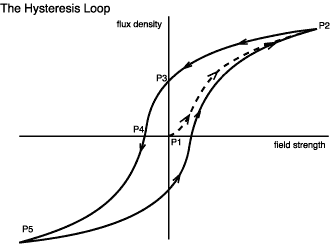
We start with an unmagnetized sample at the origin (P1) where both field strength and flux density are zero. The field strength is increased in the positive direction and the flux begins to grow along the dotted path until we reach P2. This is called the initial magnetization curve.
If the field strength is now relaxed then some curious behavior occurs. Instead of retracing the initial magnetization curve the flux falls more slowly. In fact, even when the applied field is returned to zero there will still be a remaining (remnant or remanent) flux density at P3. It is this phenomenon which makes permanent magnets possible.
To force the flux to go back to zero we have to reverse the applied field (P4). The field strength here is called the coercivity. We can then continue reversing the field to get to P5, and so on round this type of magnetization curve called a hysteresis loop.
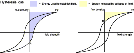
What is the significance of this from the point of power losses? It is that we have had to expend energy in order to set up the remnant flux. To show this more clearly we'll look at separate figures below. The area (shown shaded) between the B-H curve and the B axis represents the work done (per unit volume of material).
W = 0∫BH dB J m-3
You can see that the energy required to 'pump up' the core by moving from P1 to P2 is more than that which it returns when going from P2 to P3. This is evocatively termed inelastic behaviour. You could look at this another way by thinking about the 'back emf' which opposed the initial increase in coil current. The emf generated is always proportional to the change in flux; but the flux changes less on the 'way down' than it does going up.
We can go a stage further and deduce that the total power lost over one complete cycle is proportional to the area within the hysteresis loop.
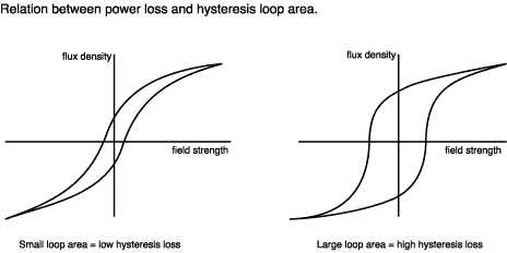 The
left hand curve shows a 'soft' magnetic material such as silicon steel.
Its area is small so it's ideal for a low loss transformer core. The
material on the right hand curve is 'hard' magnetic. Its large area is
commonly seen in materials such as Alnico (an iron/cobalt/nickel alloy)
used for permanent magnets.
The
left hand curve shows a 'soft' magnetic material such as silicon steel.
Its area is small so it's ideal for a low loss transformer core. The
material on the right hand curve is 'hard' magnetic. Its large area is
commonly seen in materials such as Alnico (an iron/cobalt/nickel alloy)
used for permanent magnets.
By the way, because this effect is related to an area, hysteresis loss is roughly proportional to the square of the working flux density. In fact, the non-linearities will, for transformer iron, reduce this to about B1.6. The particular value for a given material is called the Steinmetz exponent, n. Unfortunately, I've yet to see a data sheet which states n directly. For an iron core device it is sometimes assumed to be 1.6. For ferrite grade 3C8 it is 2.5. Data sheets sometimes have graphs of loss versus flux density on a log scale. These can be used to estimate n.
Because a hysteresis loss is incurred each time the core cycles, from positive to negative values of B, the loss rate (watts) is directly proportional to the frequency of operation, f (Hz). We can combine these proportionalities in a single formula for the hysteresis loss:
Ph = Kh×f×Bn watts m-3Where Kh also depends on the particular core material. You can build a simple circuit to display hysteresis.
By the way, this tells us why it really isn't advisable to subject a transformer to a voltage (and hence flux) overload - it's going to get hot before you go very far :-(
[Top of page]
Eddy current loss
Eddy current losses occur whenever the core material is electrically
conductive. This is intuitively obvious if you consider that the magnetic
field is contained within a circuit formed by the periphery of the core in
the same way as it is contained within a turn on the windings. Around that
periphery a current will be induced in the same way as it is in an ordinary
turn which is shorted at its ends.
In any resistive circuit the power is proportional to the square of the applied voltage. The induced voltage is itself proportional to f×B and so the eddy losses are proportional to f2B2.
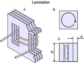
The above figure shows how the idea of lamination is used to reduce the power losses caused by eddy currents in mains transformers. The same principle applies to motors and generators too. Using a solid iron core (as in cross-section B) results in a large circulating current. So, instead, the core is made up of a stack of thin (~0.5 millimetre) sheets (cross section C). Here I have shown only four laminations but there will normally be many more. The lines of magnetic flux can still run around the core within the plane of the laminations. The situation for the eddy currents is different. The surface of each sheet carries an insulating oxide layer formed during heat treatment. This prevents current from circulating from one lamination across to its neighbours.
Clearly, the current in each lamination will be less than the very large current we had with the solid core; but there are more of these small currents. So have we really won? The answer is yes, for two reasons.
Power loss (the reduction of which is our aim) is proportional to the square of induced voltage. Induced voltage is proportional to the rate of change of flux, and each of our laminations carries one quarter of the flux. So, if the voltage in each of our four laminations is one quarter of what it was in the solid core then the power dissipated in each lamination is one sixteenth the previous value. Hurrah!
But wait; it gets better. Look at the long thin path that the eddy current takes to travel round the lamination. Suppose we made the laminations twice as thin (we halved d1). The path length of the current isn't much changed; it's still about 2×d2. However, the width of the path has halved and therefore its resistance will double and so the current will be halved. The bottom line is that eddy current loss is inversely proportional to the square of the number of laminations.
This idea of dividing up the iron into thin sections is carried a stage further in the iron dust cores. Here the iron is ground into a powder, mixed with some insulating binder or matrix material and then fired to produce whatever shape of core is required. These cores can function at several megahertz but their permeability is lower than solid iron.
[
Top of page]
PW = nPC / 2where PW is the copper loss, PC is the iron loss and n is the Steinmetz exponent for the core material.
[Top of page]