
Abstract
A solute transport experiment was carried out on 1-m long and 30-cm diameter undisturbed
saturated soil columns. Prior to the analysis of the BTCs, three different calibration methods
which
relate impedance, measured with TDR (Time Domain Reflectometry), to resident solute
concentration, were compared. The three procedures were compared for estimating the
impedance,
Zo, associated with the tracer concentration of the inlet solution, Co,
and
evidence for their validity for some particular conditions is given. The first calibration method
comprises the application of a solute pulse for a long enough time upon the assumption that the
solute will be distributed uniformly in the entire profile within that time:
Introduction
Investigations on solute transport in subsurface porous media require numerical models and
experimental data. Although a vast amount of complex mathematical flow and transport models
exist,
reliable predictions of flow and transport processes in natural, heterogeneous soils can only be
made
if appropriate values for the flow and transport parameters are available. To date, the limiting
step in
our understanding of field-scale solute transport is a lack of reliable and sufficient data (Knight,
1988).
In the past, collection of tracer data has been accomplished by the analysis of the
column effluent using a variety of tracers (e.g., van Genuchten and Wierenga, 1977;
Seyfried and Rao, 1987), by the analysis of the soil water extracted by means of solution
samplers (Wierenga and van Genuchten, 1989), or by soil coring and subsequent sampling of
the soil water (Bresler and Laufer, 1974; Bond et al., 1982). A major drawback of solution
samplers is the disruption of the flow path of the dissolved chemical at high suction (van der
Ploeg
and Beese, 1977), their limited use at low water contents due to the air entry pressure of the
ceramic cups, and the fairly small sampling volume which increases the variability of the
measurements (Hansen and Harris, 1975). Furthermore, the concentration profiles derived from
solution samplers are believed to represent flux concentrations, although it may also represent
resident concentrations or anything in between (Parker and van Genuchten, 1984). Erroneous
interpretation of the concentration mode may lead to gross under prediction or over prediction of
the solute behavior. Also, the soil water that is collected by solution samplers most probably
represents mobile water whereas water in immobile water regions may not be detected (van
Genuchten and Wierenga, 1977). As opposed to solution samplers, solute concentrations
obtained
with soil coring undoubtedly represent resident concentration. Unfortunately, soil coring is
destructive, time consuming, and provides only a limited temporal resolution of the tracer
distribution.
Recently, several authors have discussed the large potentials of TDR for measuring tracer
movements in laboratory soil columns as well as in field conditions (Kachanoski et al., 1992;
Wraith et al., 1993; Vanclooster et al., 1993; Mallants et al., 1994a; Ward et al., 1994). There are
many potential advantages of using TDR. Since the thickness of the TDR probes usually is only
a
few millimeters, it is essentially a non-destructive monitoring technique and the flow path of the
tracer is not or only minimally disturbed. TDR measures total resident concentration from both
mobile and immobile water regions for a sampling volume with a well defined geometry. TDR
allows data collection of both water content and salt concentration at a high spatial and temporal
resolution. Automation of the TDR has made it even more powerful for use in the laboratory and
even more so in field applications at remote sites (Heimovaara and Bouten, 1990). Possible
disadvantages of TDR include: only applicable to non-reactive tracers and low electrical
conductivity soils; for horizontally installed probes the calibration may be problematic even in
steady-state flow conditions (this paper).
Applications with TDR in the area of contaminant hydrology have been reported for
vertically (Kachanoski et al., 1992; Elrick et al., 1992) as well as for horizontally (Vanclooster et
al., 1993; Mallants et al., 1994a; Ward et al., 1994, Vanclooster et al., 1995) installed probes.
Most
of these studies were carried out on sandy or loamy sand soils with a low percentage of clay and
silt and without distinct macropores. These relatively favorable conditions allowed the authors to
adopt simple hypotheses for the water flow and solute transport and also for the calibration. For
instance, in the study of Ward et al. (1994), calibration constants for all horizontally installed
TDR
probes were based on the numericalconvolution of a measured pulse response with a theoretical
step function input to obtain the
theoretical step response. This approach assumes that all the mass injected could be traced back
with the TDR probes which implies an almost perfect mass recovery. Within the soil volume of
interest, i.e. the soil column, flow was relatively homogeneous such that the sampling volume of
the TDR probe represents the average resident solute concentration at a fixed depth.
Consequently, the requirement of complete mass recovery could be fulfilled. An exception is the
study by Mallants et al. (1994) where a large number of macropores was present in a sandy loam
soil containing 13% clay in the upper Ap horizon. This study showed that for macroporous soils
the TDR sampling volume may be too small to accurately measure the average concentration
across the soil column. As a result, the convalution procedure applied by Ward et al. (1994)
could
not be adopted. The heterogeneity of the flow field within the soil column required the use of an
alternative calibration methodology. Appropriate calibration constants were obtained by the
addition of a second, step function input until C = Co at the detection volume. This
is a prerequisite for relating the TDR impedance readings, Z, to resident solute concentrations.
For
instance, when the solute is applied continuously as a step function input, than the TDR reading
Z = Zo can be equated to the known solute concentration Co at time t
when the solute front has moved below the TDR probes. However, if zones of low permeability
and stagnant water are present within the sampling volume of the TDR probe, the solute may
require a long time before it has spread uniformly, hence requiring a very long (thus impractical)
application time of the solute. The success or failure of the TDR technique to accurately predict
solute concentrations therefore heavily depends on the appropriateness of the calibration
procedure used. In fact, this is also true for the ECa measurements made using
conventional four-electrode salinity probes (Rhoades et al., 1989).
In the present study we will compare three different methods for relating TDR impedance
readings to solute concentrations based on data measured at six different depths
in l-m long and 30-cm
diameter saturated undisturbed soil columns. First, the accuracy of the numerical integration
procedure to estimate calibration constants from a pulse function input of tracer (method
proposed
by Ward et al., 1994) will be evaluated. Next, the validity of an independently measured
relationship
between the bulk soil electrical conductivity (ECa) and the electrical conductivity of
the water phase
(ECw) for the prediction of solute concentrations in undisturbed soil will be
examined. Values for
the calibration constants, Zo, obtained with these two methods will be compared
with impedance data
collected for a solute application time that was long enough to satisfy the condition
Material and methods
Experimental design
Flow and solute transport processes were examined on 30 undisturbed soil columns taken one
meter
apart at the Bekkevoort experimental field, east of Leuven (Belgium). The field plot was located
in
an orchard and the transect was chosen in between two rows of trees. The surface in between the
trees
was covered with grass. Within the first meter of the soil profile, three different horizons were
identified. The thickness of the layers remained fairly constant along the transect. The average
thickness of the Ap horizon is 25 cm whereas the mean thickness of the Cl and C2 horizons is 30
and
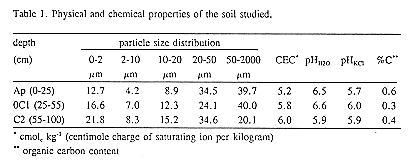
45 cm, respectively, with a sharp boundary between all soil layers. Physical and chemical
properties
of each soil horizon are listed in TABLE 1. Clay content increased
from 12.7% in the Ap horizon (0-25
cm) to 16.7 % in the C1 (25-SScm) and 21.8% in the C2 (SS-IOO cm) horizon. The Ap and Cl
are
pedogenetically identical, i.e. colluvial material, whereas the C2 is an old textural B horizon. The
soil
was classified as an Udifluvent (Eutric Regosol), with a large number of macropores throughout
the
profile. The macropores consisted mainly of decayed root channels and earthworm holes. The
columns were one meter long and 30 cm in diameter. Collection of the soil columns was done by
excavating the soil gradually in such a way that a pedestal of soil could be isolated, its diameter
slightly larger than the polyvinyl chloride (PVC) cylinder. PVC cylinders with 30-cm I.D., the
inner
side greased and the bottom end sharpened, were hydraulically driven around the soil pedestals.
The
bottom of the soil column was cut off by means of a steel plate, sharpened at one side. The plate
was
driven pneumatically under the PVC cylinder, isolating the soil column from the underlying soil.
Next, a PVC end cap was placed on both ends of the cylinder. This construction was lifted
hydraulically onto a truck and was transported to the laboratory.
In the same field, undisturbed 20-cm long and 20-cm diameter columns were also collected in
between the l-m long soil columns in the upper Ap soil horizon. We alsocollected 5.3-cm long
and 5-cm diameter soil cores next to the 20x20-cm columns for the Ap horizon
(60 in total). For the C1 and C2 horizon, 5.3x5-cm soil cores (60 samples for each horizon) were
taken exactly below the 5.3x5-cm cores' sampling locations for the Ap horizon, at depths of 50
and
90 cm, respectively. Solute transport experiments using 20-cm long columns were carried out to
investigate the applicability of TDR for measuring transport behavior at the shallow depth
(Mallants
et al., 1994a). Water content at zero pressure and bulk density were determined using the
5.3x5-cm
soil cores.
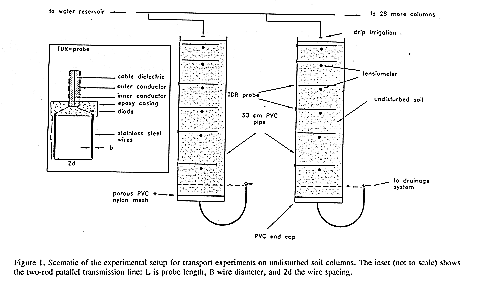
Once in the laboratory, a perforated plate was attached to the bottom end of the 1-m long
columns. On top of the perforated plate we glued a nylon-type mesh which allowed the
application
of a suction up to 70 mbar (FIGURE 1). This assembly was
attached to the bottom of the column together
with an enclosed drainage system. Drainage water from this system could be collected in small
sampling bottles via a poly-ethylene (PET) tube. The system also allowed to maintain a
watertable
at the bottom of the column or to regulate suction at the bottom of the column, while increasing
of
the water level allowed to mimic a water table inside the soil column. Water could be applied at
the
top of the columns by means of a constant rate drip irrigation system. To reduce crust formation
on
the soil surface, a 1-cm thick fiberwool cover was put on top of the soil surface. The maximum
depth
the water was allowed to pond was 1 cm. A second independent drip irrigation line was
constructed
for the application of the tracer. In this way, we could easily switch from solute free water to the
tracer solution.
Water content,
Transport experiments
Solute transport processes were monitored in saturated conditions. The soil columns were
saturated
from the bottom by gradually increasing the water level in the drainage tube in order to minimize
the
inclusion of air pockets. When the columns were completely saturated, solute free water was
applied
through the drip irrigation system at a rate large enough to generate ponding. The groundwater
level
was again established at the bottom of the soil column. As soon as steady state flow conditions
were
obtained, the application of solute free water was interrupted and the remaining water allowed to
infiltrate. Next, a 7x10⁻³ M CaCl2 solution was applied for a period of
at least 79 hr until the whole
soil column was saturated with the applied solution. Then, solute free water was applied again to
the
surface until the initially measured impedance, Zi, was again reached. The
motivation for using such
a long application time for the pulse function input was the evaluation of different calibration
procedures. Only if the column could be saturated with the tracer solution at all observation
depths,
i.e. C = CO (which is equivalent to
Calibration of the solute concentration-impedance
relationship
Solute concentrations can be deduced from TDR-based estimates of the bulk electrical
conductivity as was shown by a number of authors (Kachanoski et al., 1992; Wraith et al.,
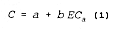
1993). A linear relationship is generally observed between the resident solute concentration, C
(g/cm3), and the bulk soil electrical conductivity, ECa, for water
contents ranging from dry to
saturation and salinity levels from 0 to 50 dS/m (Diels et al., 1994; Ward et al., 1994):
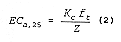
where a and b are calibration constants. The bulk soil electrical conductivity at ° C,
ECa,25 (dS/m), can be related to the impedance of an electromagnetic wave, Z
(
where Kc is the cell constant of the TDR probe (m-1), and
ft a temperature correction factor.
Once we accept EQUATIONS 1 and 2,
i.e., C ~ Z-1, the calibration is in fact not a unique problem for
TDR, but a general problem for any EC measurement device, whether TDR, electrical
conductivity probe or electromagnetic induction method. The relative solute concentration,
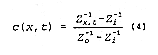
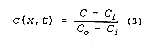
c(x,t), can be expressed as:
where Co is a reference concentration such as an input concentration and
Ci is the background
concentration. Inserting EQUATION 1 into EQUATION 3 and using EQUATION 2
results in:
where Zi> is the impedance before application of the tracer solution and
Zo, is the impedance
associated with the concentration of the inlet solution, Co. As can be seen from EQUATION 4, all constants
drop out and a solute BTC could be derived if appropriate values of Zx,t,
Zi, and Zo can be obtained.
Values for the background impedance, Zi, and the impedance throughout the course
of the transport
experiment, Zx,t, can be readily obtained. Values of Zo can be
obtained in a number of ways. For
homogeneous soils, values of Zo can be related to Co as described
below:
1. Continuous solute application
This is a most commonly used calibration method. For a continuous solute application,
Zo can be
easily related to the input solution concentration Co after a long enough time when
solutes are
distributed uniformly in the soil profile. A disadvantage of this technique is that for solute
applications in long soil columns or in the field, an impractically large amount of tracer solution
may
be required. Previous applications with this methodology have been reported by Rhoades (1981)
and
Rhoades et al. (1989) to establish ECa-ECw-
2. Pulse function input
When a single pulse of input of duration time to is applied to the surface, C is less
than Co for
relatively small t and large x. Integrating EQUATION 4 from t = 0
to t =
As long as Zi is known, Zo can be determined by evaluating the area
of measured impedance
(Vanclooster et al., 1993; Ward et al., 1994). Note that this method assumes that the TDR detects
the
same amounts of solutes as those applied on the soil surface.
3. Experimentally determined ECa-ECw
relationship
Based on EQUATION 2, the TDR measured soil impedance, Z, can
be used to calculate the bulk soil
electrical conductivity, ECa, provided the cell constant for the TDR probe,
Kc, is known. The next
step is to relate ECa, to the electrical conductivity of the water phase,
ECw, for a given soil water
content,
with
Although all of the above three methods have both advantages and disadvantages when applied
to undisturbed soil, we applied these procedures to the TDR measurements made in 1-m long
undisturbed soil columns in order to find appropriate calibrations for undisturbedsoils.
Results and discussion
All three calibration procedures were applied to the measured Z vs. time data in order to find the
most
appropriate calibration for our particular soil which would lead to meaningful resident
concentration
distributions. As will be shown in the following sections, each calibration method has its
particular
difficulties when applied to data obtained from undisturbed soil.
Application of a tracer solution for a long enough time until C = Co everywhere
seems a very
simple and attractive method for the determination of the calibration constant Zo.
Analysis of the
impedance vs. time data, Zx,t, revealed that saturation of the soil with the tracer
solution was difficult
to obtain, especially for the deeper depths. Although we found
a quick drop of the impedance after the start of the solute application, even so at deeper
observation
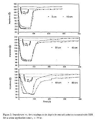
depths, the remaining part of the Z versus time curve often showed long tailing (FIGURE 3). The fast
decrease of Z is probably due to the existence of macropores (see also Mallants et al., 1993;
Mallants
et al., 1994a) which allow the tracer to move quickly downward, bypassing soil zones that are
still
solute free. The subsequent tailing of the Zx,t, curve is presumably caused by
physical nonequilibrium
effects in the transport process: the solute slowly diffuses from the higher concentration zones,
usually the larger pores, to the low concentration zones, mostly the smaller pores, dead-end pores
and
the less permeable soil matrix (recall that clay percentage in the lower C2 horizon is
approximately
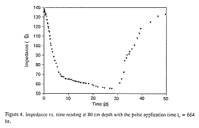
22%). These nonequilibrium effects can be very extreme, as can be seen in FIGURE 4. For an observation
depth of 80 cm, the impedance decreases from approximately 140
An alternative calibration method consisted in the numerical integration of the response to a
long pulse function input in order to derive Zo according to EQUATION 5. To test this calibration procedure,
estimates of Zo following EQUATION 5 were
compared with measured values of Zo for those locations
where
Since it is reasonable to assume that the flow processes become more homogeneous at larger
depths, the estimates of Zo presumably will not become less accurate for greater
depths. We
therefore decided that for all those depths were
where
where p the proportion of the electromagnetic energy. For
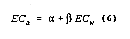
The third calibration method tested was based on experimentally determined
ECa-ECw
relationships for different water contents,
It is remarkable that, at least for the first two observation (5 and 15 cm), differences between
values for
Zo are small. For the other depths, differences between method (2) and (3) increase.
Since the
ECa-ECw-
i.e., ECs = 0.278 dS/m for the Ap and 0.485 dS/m for the C2 horizon,
respectively. One can
doubt
about the validity of EQUATION 9 for soils with completely
different mineralogy and texture than the
ones
used to derive the relationship, but at least the relation between ECs and clay
percentage indicates
that
soil horizons with different clay content will have a different ECs. The value of
ECs obtained
from
regression analysis (which is in fact equivalent to the
Conclusions
The Zx,t data measured with TDR in l-m long undisturbed soil for a long
application time of the
tracer
solution was evaluated in terms of three different calibration procedures. These calibrations are
necessary to obtain the characteristic impedance Zo associated with the
concentration of the inlet
solution, Co. The value of Zo is required to interpret the
Zx,t data in terms of solute resident
concentration BTCs. Although application of the tracer solution for a time long enough to
saturate
the soil completely (C = Co or
The second calibration method tested was based on the numerical integration of the
(Z-1 - Zi-1)
curve. Based on comparisons of measured and predicted Zo values at depths of x =
5 cm, this
method
performed good. With flow processes becoming more homogeneous at deeper depths in the soil
profile, it was concluded that this procedure could be applied to the deeper depths where
In the third calibration method we estimated Zo from an experimentally
determined ECa-ECw
relationship. Based on ECa-ECw curves for different water contents,
an ECa-ECw-
References
Bond, W. J., B.N. Gardiner, and D.E. Smiles. 1982. Constant-flux adsorption of a Tritiated
Calcium Chloride solution by a clay soil with anion exclusion. Soil Sci. Soc. Am. J., vol.
46, 1133-1137.
Bresler, E., and A. Laufer. 1974. Anion exclusion and coupling effects in nonsteady transport
through
unsaturated soils: 11. Laboratory and numerical experiments. Soil Sci. Soc. Am. Proc.,
vol. 38,
213-218.
Diels, J., Md. A.A. Sarkar, D. Mallants, M. Vanclooster, and J. Feyen. 1994. Calibration of time
domain
reflectometry for the measurement of soil water content and salt concentration. Submitted to
Irrigation
Science.
Elrick, E.E., R.G., Kachanoski, E.A., Pringle, and A. Ward. 1992. Parameter estimation of field
scale transport
models based on time domain reflectometry measurements. Soil Sci. Soc. Am. J., 56,
1663-1666.
Hansen, E.A.. and A.R. Harris. 1975 Validity of soil-water samples with porous ceramic cups.
Soil Sci. Soc.
Am. Proc., 39, 528-536.
Heimovaara, T.J. 1993. Time domain reflectometry in soil science: theoretical backgrounds,
measurements and
models. Ph.D. thesis, University of Amsterdam, The Netherlands, 169 pp.
Heimovaara, T.J. and Bouten, W., 1990. A computer-controlled 36-channel time-domain
reflectometry system
for monitoring soil water contents. Water Resour. Res., 26: 2311-2316.
Kachanoski, R.G., E. Pringle, and A. Ward. 1992. Field measurement of solute travel times using
time domain
reflectometry. Soil Sci. Soc. Am. J., vol. 56, 47-52.
Knight, J.H., 1988. Solute transport and dispersion. IN W.L. Steffen, O.T. Denmead (eds):
Flow
and transport
in the natural environment: Advances and applications. Springer-Verlag, N.Y., pp.
17-29.
Knight, J.H., 1992. Sensitivity of Time Domain Reflectometry measurements to lateral variations
in water
contents. Water Resour. Res., vol. 28, p. 2345-2352.
Mallants, D., N. Toride, M.Th. van Genuchten, and J. Feyen. 1993. Using dyes for quantifying
preferential
flow in a sandy loam soil. AGU 1993 Fall Meeting, San Francisco, CA, p. 240.
Mallants, D., M. Vanclooster, M. Meddahi, and J. Feyen. 1994a. Estimating solute transport
parameters on
undisturbed soil columns using time domain reflectometry. J. Cont. Hydrol.,
17:91-109.
Mallants, D., N. Toride, M. Vanclooster, M.Th. van Genuchten, and J. Feyen, 1994b. Using TDR
to monitor
solute transport in long undisturbed soil columns during steady saturated flow. In:
Proceedings of
the 15th
International Congress of Soil Science (Symposium Ibi Soil Physics and
the Environmental Protection), Acapulco, Mexico, July 10-16, 147-148.
Mallants, D., M. Vanclooster, and J. Feyen, 1995. Transect study on solute transport in
macroporous soil.
Hydrological Processes (in press).
Nadler, A., S. Dasberg, and I. Lapid. 1991. Time domain reflectometry measurements of water
content and
electrical conductivity of layered soil columns. Soil Sci. Soc. Am. J., vol. 55,
938-943.
Parker, J.C., and M. Tb. van Genuchten. 1984. Flux-averaged concentrations in continuum
approaches to solute
transport. Water Resour. Res., 20, 866-872.
Rhoades, J.D. 1981. Predicting bulk soil electrical conductivity vs. saturation paste extract
electrical conductivity
calibrations from soil properties. Soil Sci. Soc. Am. J., vol. 45; 42-44.
Rhoades, J. D, P.A.C. Raats, and R.J. Prather. 1976. Effects of liquid-phase electrical
conductivity, water content,
and surface conductivity on bulk electrical conductivity. Soil Sci. Soc. Am. J., vol. 40,
651-655.
Rhoades, J.D., N.A. Manteghi, P.J. Shouse, and W.l. Alves. 1989. Soil electrical conductivity
and soil salinity:
New formulations and calibrations. Soil Sci. Soc. Am. J., vol. 53, 433-439.
Seyfried, M.S., and P.S.C. Rao. 1987. Solute transport in undisturbed columns of an aggregated
tropical soil:
Preferential flow effects. Soil Sci. Soc. Am. J., vol. 51, 1434-1444.
Vanclooster, M., D. Mallants, J. Diels, and J. Feyen. 1993. Determining local-scale solute
transport parameters
using time domain reflectometry. J. Hydrol., 148, 93-107.
Vanclooster, M., D. Mallants, I. Vanderborght, I. Diels, J. Van Orshoven, and J. Feyen, 1995.
Monitoring solute
transport in a multi-layered sandy Iysimeter using time domain reflectometry. Soil Sci. Soc.
Am.
J. (in press).
van der Ploeg, R.R., and F. Beese. 1977. Model calculations for the extractions of soil water by
ceramic cups and
plates. Soil Sci. Soc. Am. J., 41, 466-470.
van Genuchten, M.Th., and P.J. Wierenga. 1977. Mass transfer studies in absorbing porous
media: 11.
Experimental evaluation with Tritium (3H2O). Soil Sci. Soc. Am.
J., vol. 41, 272-278.
Ward, A.L., R.G Kachanoski, and D.E. Elrick. 1994. Laboratory measurements of solute
transport using time
domain reflectometry. Soil Sci. Soc. Am. J. (Accepted tor publication)
Wierenga, P.J., and M.Th. van Genuchten. 1989. Solute transport through small and large
unsaturated soil
columns. Ground Water, vol. 27, 35-42.
Wraith, J.M., S.D. Comfort, B.L. Woodbury, and W.P. Inskeep. 1993. A simplified waveform
analysis approach
for monitoring solute transport using time-domain reflectometry. Soil. Sci. Soc. Am. J.,
vol. 57,
637-642.
Last modified: 06-10-98
![]() C/
C/![]() t = 0 and C = Co everywhere. For the second method, the response to a
pulse function input is convolved numerically to yield the response to a step function input from
which Zo can be readily obtained. The third method determines Zo
based on an experimentally determined ECa-ECw-
t = 0 and C = Co everywhere. For the second method, the response to a
pulse function input is convolved numerically to yield the response to a step function input from
which Zo can be readily obtained. The third method determines Zo
based on an experimentally determined ECa-ECw-![]() relationship on repacked soil. All methods compared favorably well at the first observation depth
(x = 5 cm). Deeper in the soil profile, physical nonequilibrium effects were dominating the
transport process with long equilibration times necessary to diffuse the solutes from the mobile
to
the immobile water regions. As a result, the first calibration method was only valid at shallow
depths. The second calibration procedure could be applied throughout the whole soil profile upon
the assumption that flow was homogeneous. The procedure based on the empirical
ECa-ECw-
relationship on repacked soil. All methods compared favorably well at the first observation depth
(x = 5 cm). Deeper in the soil profile, physical nonequilibrium effects were dominating the
transport process with long equilibration times necessary to diffuse the solutes from the mobile
to
the immobile water regions. As a result, the first calibration method was only valid at shallow
depths. The second calibration procedure could be applied throughout the whole soil profile upon
the assumption that flow was homogeneous. The procedure based on the empirical
ECa-ECw-![]() relationship gave surprisingly good
predictions of Zo for the upper horizon, although the simple model did not account
for the current flow through large continuous pores that were present in the soil profile.
relationship gave surprisingly good
predictions of Zo for the upper horizon, although the simple model did not account
for the current flow through large continuous pores that were present in the soil profile.![]() C/
C/![]() t = 0 for at
least one observation depth (third method). The effects of calculating inappropriate values for the
calibration parameters on solute BTCs will be illustrated for one extreme case.
t = 0 for at
least one observation depth (third method). The effects of calculating inappropriate values for the
calibration parameters on solute BTCs will be illustrated for one extreme case.![]() , and bulk soil electrical conductivity, ECa,
of the soil were monitored by TDR
probes whereas pressure head was measured with tensiometers. Both devices were installed at six
different depths (5, 15, 30, 45, 60, and 80 cm, see also FIGURE 1).
, and bulk soil electrical conductivity, ECa,
of the soil were monitored by TDR
probes whereas pressure head was measured with tensiometers. Both devices were installed at six
different depths (5, 15, 30, 45, 60, and 80 cm, see also FIGURE 1).![]() C/
C/![]() t = 0) at z = 5, 15, ...,
80 cm, then the necessary conditions
for evaluation would be fulfilled. For several soil columns. application
of the tracer solution for 79 hr was not sufficient to obtain a constant concentration (C =
Co
everywhere), even at 5 cm depth. For these columns, the solute was applied until
t = 0) at z = 5, 15, ...,
80 cm, then the necessary conditions
for evaluation would be fulfilled. For several soil columns. application
of the tracer solution for 79 hr was not sufficient to obtain a constant concentration (C =
Co
everywhere), even at 5 cm depth. For these columns, the solute was applied until ![]() C/
C/![]() t = 0 at x
= 5 cm, unless the application time became practically infeasible. For some extreme cases,
solute had to be applied for 664 hr. Therefore, the application time of the solute was different
for different columns, except for those where the application time to = 79 hr. Throughout the
experiment, water content and bulk soil electrical conductivity were measured with TDR. We
used a TEKTRONIX cable tester (TEKTRONIX, 1502B, BEAVERTON, OREGON, USA)
and multiplexed the different channels manually. The travel time of the electromagnetic wave
and the impedance Z were taken from the screen of the cable tester. Values of Z were taken at a
far distance on the reflected wave form (t
t = 0 at x
= 5 cm, unless the application time became practically infeasible. For some extreme cases,
solute had to be applied for 664 hr. Therefore, the application time of the solute was different
for different columns, except for those where the application time to = 79 hr. Throughout the
experiment, water content and bulk soil electrical conductivity were measured with TDR. We
used a TEKTRONIX cable tester (TEKTRONIX, 1502B, BEAVERTON, OREGON, USA)
and multiplexed the different channels manually. The travel time of the electromagnetic wave
and the impedance Z were taken from the screen of the cable tester. Values of Z were taken at a
far distance on the reflected wave form (t ![]()
![]() ).
).![]()
![]() ), that travels through
the soil, following Nadler et al. (1991):
), that travels through
the soil, following Nadler et al. (1991):![]()
![]()
![]() relationships for field soils using four-electrode
salinity probes.
relationships for field soils using four-electrode
salinity probes.![]() for a pulse function input leads
to
for a pulse function input leads
to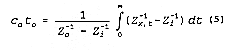
![]() . The most simple form of this relation is
. The most simple form of this relation is![]()
![]() and
and ![]() empirical parameters. It has been shown
(Rhoades et al., 1976) that the parameter
empirical parameters. It has been shown
(Rhoades et al., 1976) that the parameter ![]() represents the electrical conductivity of the solid phase of the soil (ECs), and the
parameter
represents the electrical conductivity of the solid phase of the soil (ECs), and the
parameter ![]() is
equal to T
is
equal to T![]() w (T a transmission coefficient equal to the fraction
of "mobile" water, i.e. the large
pore system, and
w (T a transmission coefficient equal to the fraction
of "mobile" water, i.e. the large
pore system, and ![]() w, the total soil water content). A more
physically based model (the "three-pathway model") was proposed by Rhoades et al. (1989)
taking into account the current carrying
capacity of the solid phase (ECs), the small pores and intraped pores
(ECws) and the larger or
continuous pores (ECwc or simply ECw). For a comparison between
empirical ECa-ECw
relationships and predicted EC,-ECW relationships based on the "three-pathway" model of
Rhoades
(1989), the reader is referred to Diels et al. (1994). The ECa-ECw
relationship used in this study was
determined for repacked Bekkevoort sandy loam soil, taken from the same transect as our soil
columns. Diels et al. (1994) used linear regression analysis to obtain intercept and slope of EQUATION 6
for sets of ECa-ECw data for three different water contents (0.12, 0.24
and 0.36 cm3cm-3) and eight
different salt concentrations. Linear relationships were found for all three water contents for
salinity
levels from 0 to 50 dS/m, with r2 ranging from 0.81 (
w, the total soil water content). A more
physically based model (the "three-pathway model") was proposed by Rhoades et al. (1989)
taking into account the current carrying
capacity of the solid phase (ECs), the small pores and intraped pores
(ECws) and the larger or
continuous pores (ECwc or simply ECw). For a comparison between
empirical ECa-ECw
relationships and predicted EC,-ECW relationships based on the "three-pathway" model of
Rhoades
(1989), the reader is referred to Diels et al. (1994). The ECa-ECw
relationship used in this study was
determined for repacked Bekkevoort sandy loam soil, taken from the same transect as our soil
columns. Diels et al. (1994) used linear regression analysis to obtain intercept and slope of EQUATION 6
for sets of ECa-ECw data for three different water contents (0.12, 0.24
and 0.36 cm3cm-3) and eight
different salt concentrations. Linear relationships were found for all three water contents for
salinity
levels from 0 to 50 dS/m, with r2 ranging from 0.81 (![]() = 0.12)
to 0.99 (
= 0.12)
to 0.99 (![]() = 0.36). The data analyzed
by Diels et al. (1994) did not show any significant curvilinearity for low concentrations
(ECw ~ 0.5 dS/m) of the electrolytes in the soil solution. In the same study, values
for the cell constant Kc were
derived in a way similar to Heimovaara (1993). Based on the previously determined
ECa-ECw
relationships, we derived a continuous ECa-ECw-
= 0.36). The data analyzed
by Diels et al. (1994) did not show any significant curvilinearity for low concentrations
(ECw ~ 0.5 dS/m) of the electrolytes in the soil solution. In the same study, values
for the cell constant Kc were
derived in a way similar to Heimovaara (1993). Based on the previously determined
ECa-ECw
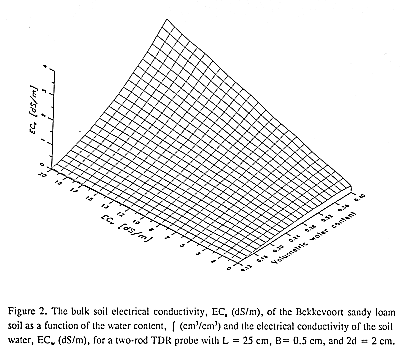
relationships, we derived a continuous ECa-ECw-![]() surface (FIGURE 2). Based on these
ECa-ECw-
surface (FIGURE 2). Based on these
ECa-ECw-![]() relationships we can determine EC
relationships we can determine EC![]() .
.![]() to 65
to 65
![]() in about 7 to 8 days. For
the next 20 days, however, Z drops only up to 55
in about 7 to 8 days. For
the next 20 days, however, Z drops only up to 55 ![]() . It is clear that even
after almost 30 days of solute
application, the solute concentration has not yet reached the concentration of the inlet solution, or
C < Co. This shows that the diffusion of solute from the mobile water region to the
immobile or
stagnant water region can be very slow. It waspractically impossible to apply the solute for all
columns for more than 30 days. For this reason, we
could not use the final impedance values for Z to estimate Zo at the deeper
observation depths, since
C < Co. For the extreme case of nonequilibrium transport such as the example
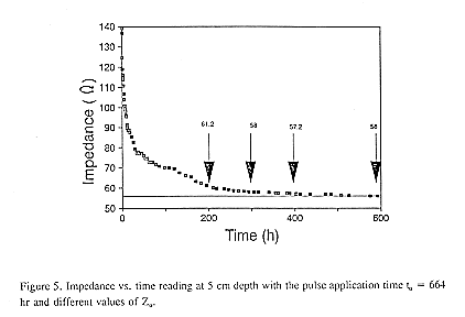
shown in FIGURE 5, the
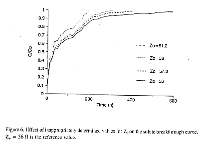
BTCs can be very susceptible to values of Zo that are incorrectly measured, i.e. Z <
Zo. To illustrate
this effect, the extreme case of FIGURE 5 will be discussed. At a
depth of 5 cm, it took 664 hr to
completely saturate the soil with the tracer solution, i.e.
. It is clear that even
after almost 30 days of solute
application, the solute concentration has not yet reached the concentration of the inlet solution, or
C < Co. This shows that the diffusion of solute from the mobile water region to the
immobile or
stagnant water region can be very slow. It waspractically impossible to apply the solute for all
columns for more than 30 days. For this reason, we
could not use the final impedance values for Z to estimate Zo at the deeper
observation depths, since
C < Co. For the extreme case of nonequilibrium transport such as the example
shown in FIGURE 5, the
BTCs can be very susceptible to values of Zo that are incorrectly measured, i.e. Z <
Zo. To illustrate
this effect, the extreme case of FIGURE 5 will be discussed. At a
depth of 5 cm, it took 664 hr to
completely saturate the soil with the tracer solution, i.e. ![]() C/
C/![]() t
= 0, for which the final impedance
was Zo = 56
t
= 0, for which the final impedance
was Zo = 56 ![]() . At t = 400 hr, Z = 57.2
. At t = 400 hr, Z = 57.2 ![]() , a value close to Zo, while at t = 300 hr Z = 58
, a value close to Zo, while at t = 300 hr Z = 58 ![]() and for
t = 200hr Z = 61.2
and for
t = 200hr Z = 61.2 ![]() . These values were selected to show the effects of
cutting off the Z vs time
curve too soon, which is equivalent to applying tracer solution for a too short time. FIGURE 6 shows the
BTCs based on EQUATION 4 for the reference value
Zo = 56
. These values were selected to show the effects of
cutting off the Z vs time
curve too soon, which is equivalent to applying tracer solution for a too short time. FIGURE 6 shows the
BTCs based on EQUATION 4 for the reference value
Zo = 56 ![]() and the three "error" values of Zo.
Cutting
off the Zx,t data too soon results in earlier breakthrough and less tailing. The effect
of less tailing of
the BTC on the solute transport parameters can be evaluated by fitting solutions of the transport
equation to the observed data (not shown here).
and the three "error" values of Zo.
Cutting
off the Zx,t data too soon results in earlier breakthrough and less tailing. The effect
of less tailing of
the BTC on the solute transport parameters can be evaluated by fitting solutions of the transport
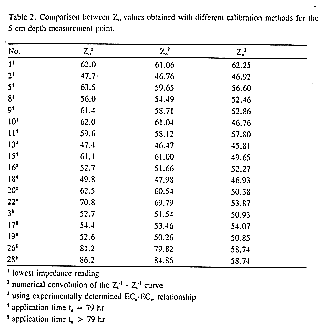
equation to the observed data (not shown here).![]() C/
C/![]() t = 0. The results given in TABLE 2 illustrate that estimates of ZO using the
numerical
convolution procedure only minimally deviate from the presumed correct value of
Zo.
t = 0. The results given in TABLE 2 illustrate that estimates of ZO using the
numerical
convolution procedure only minimally deviate from the presumed correct value of
Zo.![]() C/
C/![]() t
t ![]() 0, the numerical integration of the pulse
input function is a valid procedure to estimate values of Zo. We note again that this
procedure
assumes that all the mass is recovered at the detection volume of the TDR. In a similar study
using
a set of 20x20 cm columns, Mallants et al. (1994; 1995) indicated that the presence of
preferential
flow paths in soil columns may force the solute to bypass the detection volume of the TDR
probes
and the condition of mass recovery might not be met. If such flow phenomena are suspected to
occur in the soil being investigated, the first calibration method has to be used. The problem of a
too small detection volume is related to the theory
of a Representative Elementary Volume (REV). In macroporous soil, the sample volume of the
TDR
probes may not contain a representative amount of the local variations in the flow properties.
Sampling
volumes for TDR probes can be calculated in the following way. Consider TDR probes
consisting of two
parallel waveguides, with the distance between the center of the rods, 2d, equal to 2.5 cm (see
inset FIGURE 1). When the diameter of the stainless steel rods, B,
equals 0.5 cm, the effective sampling volume
of the
TDR probe can be estimated from (see Knight, 1992):
0, the numerical integration of the pulse
input function is a valid procedure to estimate values of Zo. We note again that this
procedure
assumes that all the mass is recovered at the detection volume of the TDR. In a similar study
using
a set of 20x20 cm columns, Mallants et al. (1994; 1995) indicated that the presence of
preferential
flow paths in soil columns may force the solute to bypass the detection volume of the TDR
probes
and the condition of mass recovery might not be met. If such flow phenomena are suspected to
occur in the soil being investigated, the first calibration method has to be used. The problem of a
too small detection volume is related to the theory
of a Representative Elementary Volume (REV). In macroporous soil, the sample volume of the
TDR
probes may not contain a representative amount of the local variations in the flow properties.
Sampling
volumes for TDR probes can be calculated in the following way. Consider TDR probes
consisting of two
parallel waveguides, with the distance between the center of the rods, 2d, equal to 2.5 cm (see
inset FIGURE 1). When the diameter of the stainless steel rods, B,
equals 0.5 cm, the effective sampling volume
of the
TDR probe can be estimated from (see Knight, 1992):![]()
![]() = r/d the dimensionless radius of the cylindrical sampling volume,
= r/d the dimensionless radius of the cylindrical sampling volume,
![]() = B/d, and
q is defined as:
= B/d, and
q is defined as:![]()
![]() = 0.4, we can
calculate that for p =
0.95, 95%
of the energy is within a cylinder of radius 3.3d. For the configuration used in this study, we find
a
cylinder of influence with diameter 6.6 cm. We note that this theory was applied to
measurements of
water content,
= 0.4, we can
calculate that for p =
0.95, 95%
of the energy is within a cylinder of radius 3.3d. For the configuration used in this study, we find
a
cylinder of influence with diameter 6.6 cm. We note that this theory was applied to
measurements of
water content, ![]() (Knight, 1992). We assume, at this point, that it also holds
for measurements of
electrical conductivity, EC. For TDR probes that are 25 cm long (this study), the cross-sectional
sampling
area is
(Knight, 1992). We assume, at this point, that it also holds
for measurements of
electrical conductivity, EC. For TDR probes that are 25 cm long (this study), the cross-sectional
sampling
area is ![]() 165 cm2 or 23% of the total cross-sectional area.
Thus, in the study presented here,
almost one
fourth of the total potential cross-sectional flow area could be sampled. For the 1-m long
columns
investigated here, this seems sufficient to trace the complete solute pulse. Unlike the severe
preferential
flow effects for short columns in the study of Mallants et al. (1994), longer columns tend to
reduce the
effects of preferential flow because macropores most likely will not be continuous from top to
bottom
of the column. As a result, lateral spreading of solute is enhanced and flow becomes more
homogeneous
throughout the profile, as was already demonstrated by Mallants et al. (1994b). This allows the
application of calibration methods such as the numerical convolution discussed here.
165 cm2 or 23% of the total cross-sectional area.
Thus, in the study presented here,
almost one
fourth of the total potential cross-sectional flow area could be sampled. For the 1-m long
columns
investigated here, this seems sufficient to trace the complete solute pulse. Unlike the severe
preferential
flow effects for short columns in the study of Mallants et al. (1994), longer columns tend to
reduce the
effects of preferential flow because macropores most likely will not be continuous from top to
bottom
of the column. As a result, lateral spreading of solute is enhanced and flow becomes more
homogeneous
throughout the profile, as was already demonstrated by Mallants et al. (1994b). This allows the
application of calibration methods such as the numerical convolution discussed here.![]() . The expected calibration
constant, Zo for a known
concentration of the inlet solution, Co, was obtained by first computing
ECa, for a given ECw
(for a
given temperature, unique relationships exist between ECw and the concentration of
a solute, say
Co).
Next, values of ECa are transformed to impedance, Z (or Zo if C =
Co) following EQUATION 2.
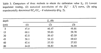
Results are
illustrated in TABLE 3 for one column where, in addition, values of
Zo obtained with the two
other
calibration methods are also presented.
. The expected calibration
constant, Zo for a known
concentration of the inlet solution, Co, was obtained by first computing
ECa, for a given ECw
(for a
given temperature, unique relationships exist between ECw and the concentration of
a solute, say
Co).
Next, values of ECa are transformed to impedance, Z (or Zo if C =
Co) following EQUATION 2.
Results are
illustrated in TABLE 3 for one column where, in addition, values of
Zo obtained with the two
other
calibration methods are also presented.![]() relationship was determined only for the soil representative for the upper Ap horizon (0-25 cm),
it is
reasonable to find discrepancies for soil layers that have other physico-chemical properties. As
the clay
content increases from 13% in the Ap horizon to 22 % in the C2 horizon (see TABLE 1), the
intercept of
the ECa-ECw curve will also increase. This is because the intercept
can be interpreted as being
equal to
ECs, the electrical conductivity of the solid phase (Rhoades et al., 1989). We
evaluated the effect
of
increasing clay content on ECs following FIGURE 5
from Rhoades et al. (1989):
relationship was determined only for the soil representative for the upper Ap horizon (0-25 cm),
it is
reasonable to find discrepancies for soil layers that have other physico-chemical properties. As
the clay
content increases from 13% in the Ap horizon to 22 % in the C2 horizon (see TABLE 1), the
intercept of
the ECa-ECw curve will also increase. This is because the intercept
can be interpreted as being
equal to
ECs, the electrical conductivity of the solid phase (Rhoades et al., 1989). We
evaluated the effect
of
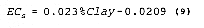
increasing clay content on ECs following FIGURE 5
from Rhoades et al. (1989):![]()
![]() parameter from EQUATION 6 was 0.363 dS/m (for
parameter from EQUATION 6 was 0.363 dS/m (for ![]() = 0.36
cm3 cm-3. Owing to the typical shape of
the ECa-ECw curves (see for instance FIGURE 8 from Rhoades et al., 1989), the relative contribution
from
ECs to ECa is larger for lower values of ECw. Because
we used rather low concentrations (the
electrical conductivity of the tracer solution was approximately 2.3 dS/m), effects of changing
ECs might have been important enough to partly explain the observed differences
between Zo from
method (2) and (3). Another explanation for the discrepancies might be the differences in bulk
density
(1.42 g/cm3 for Ap vs. 1.52 g/cm3 for C2), since the
electromagnetic wave travels mainly via the large, continuous pores, at least at normal levels of
water
content (Rhoades et al., 1989). However, the surprisingly good agreement between
Zo at x = 5
and
x = 15 cm (TABLE 2) for both methods suggests that soil structure
(the complicated arrangement
of
interconnected macropores and micropores and the direct particle to particle contact) does not
seem
to be so important if we want to relate ECa to ECw. To further test the
performance of the
ECa-ECw-
= 0.36
cm3 cm-3. Owing to the typical shape of
the ECa-ECw curves (see for instance FIGURE 8 from Rhoades et al., 1989), the relative contribution
from
ECs to ECa is larger for lower values of ECw. Because
we used rather low concentrations (the
electrical conductivity of the tracer solution was approximately 2.3 dS/m), effects of changing
ECs might have been important enough to partly explain the observed differences
between Zo from
method (2) and (3). Another explanation for the discrepancies might be the differences in bulk
density
(1.42 g/cm3 for Ap vs. 1.52 g/cm3 for C2), since the
electromagnetic wave travels mainly via the large, continuous pores, at least at normal levels of
water
content (Rhoades et al., 1989). However, the surprisingly good agreement between
Zo at x = 5
and
x = 15 cm (TABLE 2) for both methods suggests that soil structure
(the complicated arrangement
of
interconnected macropores and micropores and the direct particle to particle contact) does not
seem
to be so important if we want to relate ECa to ECw. To further test the
performance of the
ECa-ECw-![]() relationship for predicting
Zo for a given Co, we computed Zo for those columns
that reached
an equilibrium condition at the first observation depth (x = 5 cm), i.e. C = Co. TABLE 2 lists
values
of Zo according to the three calibration procedures. At least nine out of eighteen
values are close
to or relatively close to the measured value of Zo. This proves that at least for a
subset of the
date
the ECa-ECw-
relationship for predicting
Zo for a given Co, we computed Zo for those columns
that reached
an equilibrium condition at the first observation depth (x = 5 cm), i.e. C = Co. TABLE 2 lists
values
of Zo according to the three calibration procedures. At least nine out of eighteen
values are close
to or relatively close to the measured value of Zo. This proves that at least for a
subset of the
date
the ECa-ECw-![]() relationship is capable of giving
reasonable accurate predictions of Zo for a
given
Co, although the relationship has been determined on repacked soil.
relationship is capable of giving
reasonable accurate predictions of Zo for a
given
Co, although the relationship has been determined on repacked soil.![]() C/
C/![]() t = 0) seems
the most attractive method (no assumptions
about
the flow process or use of empirical calibration models), this study showed that it may not be
generally applicable. Slow transport of solutes through diffusion from mobile to immobile water
zones, may require a very long application time before
t = 0) seems
the most attractive method (no assumptions
about
the flow process or use of empirical calibration models), this study showed that it may not be
generally applicable. Slow transport of solutes through diffusion from mobile to immobile water
zones, may require a very long application time before ![]() C/
C/![]() t =
0. It then becomes practically
impossible to continue the application of tracer solution, especially for larger areas or relatively
deep
soil profiles. The sensitivity of the interpretation of the Zx,t data in terms of solute
BTCs was
demonstrated by cutting off the Zx,t curve at times smaller than the equilibration
time. Although
differences in Zo values were relatively small, the differences in the resulting BTCs
could not be
neglected.
t =
0. It then becomes practically
impossible to continue the application of tracer solution, especially for larger areas or relatively
deep
soil profiles. The sensitivity of the interpretation of the Zx,t data in terms of solute
BTCs was
demonstrated by cutting off the Zx,t curve at times smaller than the equilibration
time. Although
differences in Zo values were relatively small, the differences in the resulting BTCs
could not be
neglected.![]() C/
C/![]() t
t ![]() 0.
In relatively short soil columns with heterogeneous flow paths this procedure cannot be applied
because the assumption of mass conservation is difficult to fulfill.
0.
In relatively short soil columns with heterogeneous flow paths this procedure cannot be applied
because the assumption of mass conservation is difficult to fulfill.![]() surface was
generated and the values of Zo for known solute concentrations Co
and local values of
surface was
generated and the values of Zo for known solute concentrations Co
and local values of ![]() were
determined. Comparison of these Zo values with measured values at an
observation depth of x = 5 cm showed that although the ECa-ECw
relationship was determined
on
repacked soil, and thus reducing the current carrying capacity of the large
continuous pores, both values compared favorably well. This is promising since it suggests
that a proper calibration of the ECa-ECw-
were
determined. Comparison of these Zo values with measured values at an
observation depth of x = 5 cm showed that although the ECa-ECw
relationship was determined
on
repacked soil, and thus reducing the current carrying capacity of the large
continuous pores, both values compared favorably well. This is promising since it suggests
that a proper calibration of the ECa-ECw-![]() relationship on disturbed or preferably undisturbed
soil samples would be a sufficiently accurate technique to determine local values of
Zo. The
potential advantage of this method is that it allows interpretation of TDR-estimated electrical
conductivity data for transient flow conditions.
relationship on disturbed or preferably undisturbed
soil samples would be a sufficiently accurate technique to determine local values of
Zo. The
potential advantage of this method is that it allows interpretation of TDR-estimated electrical
conductivity data for transient flow conditions.