
by Henrik H. Nissen and Per Moldrup
Environmental Engineering Laboratory, Aalborg University, Aalborg, Denmark
The intention with this paper is to give a general introduction to the principles and theories behind measuring water content in soil with TDR. As relatively newcomers within this subject it is our experience that new users of the TDR technology lack a very general and easily understandable paper which makes the introduction phase to the TDR equipment shorter and much smoother. Thereby time is saved which can be used on what the majority of the users really want -- to carry out water content measurements in soil. Moreover there is a certain satisfaction knowing how the TDR equipment works, so that it does not appear as a black box to the user.
Introduction
TDR is short for Time Domain Reflectometry. An apparatus which is based on the TDR
principle launches electromagnetic waves and then measures the amplitudes of the reflections of
the waves together with the time intervals between the waves are launched and the reflections are
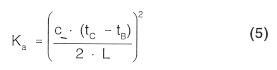
detected. The radar equipment on ships is based on TDR and will be used as an example. Radar
equipment on the ship shown in FIGURE 1 sends out
electromagnetic waves in all directions parallel to the surface of the sea.
The electromagnetic waves propagate along the surface of the sea away from the ship and the
placement of the start of the waves at different time intervals is shown as circles on FIGURE 1. If the electromagnetic waves meet any subject above
the sea surface (e.g. a rock) the waves are reflected back towards the ship where the radar
equipment pick up the reflected electromagnetic waves. By measuring (I) the time interval
between launching the electromagnetic waves and detection of the reflections, (ii) the amplitude
of the reflections and (iii) the direction of the reflections and combining this with knowledge of
the traveling speed of the waves it is possible to determine position and size of the subject that
created the reflections.
The same principles are also used in cable testing. Electromagnetic waves are launched into the
cable. Any faults on the cable change the electric properties of the cable which create reflections
of the waves (partly or total reflections depending on the type of fault). Like in the case of the
radar equipment, the equipment used for cable testing also measures the time between launching
the waves and detection of the reflections. Knowledge of the propagation velocity of the waves
makes it possible to calculate the distance to the fault. The amplitude of the reflections contains
information about the type of fault. TDR measurements of water content in soil are carried out
with the same equipment used for cable testing, a so-called metallic cable tester.
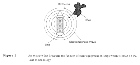
A metallic cable tester generally consists of 4 main components: a step pulse generator, a coaxial
cable, a sampler, and an oscilloscope. This is shown on FIGURE
2.
The four components will be described briefly in the following.
The step pulse generator produces the electromagnetic waves. An electromagnetic wave consists
of both an electric and a magnetic part. Most soils are non-magnetic and the magnetic part of the
waves is therefore usually without interest. However the electric part is influenced by the soil
properties and, especially, the influence is a function of the soil-water content. This will be
discussed later in this paper.
The electric part of the electromagnetic waves consists of sine shaped waves covering a large
frequency range, but it is not accidental which frequencies the step pulse generator produces. If a
sine shaped wave is superimposed with harmonic sine shaped waves, where the highest
frequency tends towards infinity, the result will be a perfect periodic square wave. This is what
happens in the step pulse generator, i.e., the electric parts of the electromagnetic waves
produces a periodic square wave (in this paper called a voltage step). In reality there is a
technically dependent upper limit for the highest frequency that can be produced by the step
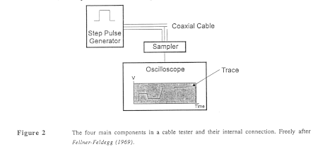
pulse generator and therefore the square waves are only approximately square. If the cable tester
is of the type Tektronix 1502B or C, which are the most commonly used in soil science, the step
pulse generator produces voltage steps as illustrated in FIGURE
3.
In this case, the voltage steps are produced by superimposing a sinus shaped wave with a ground
frequency of 16.6 kHz with harmonic sinus shaped waves up to 1.75 GHz (Tektronix,
1987). FIGURE 3 illustrates that the voltage steps are
produced in a pattern. One voltage step is transmitted over a period of 10 µs and after that
there is a pause in the transmission lasting 50 µs.
The step pulse generator and the sampler are connected with a coaxial cable also known as an
antenna wire.
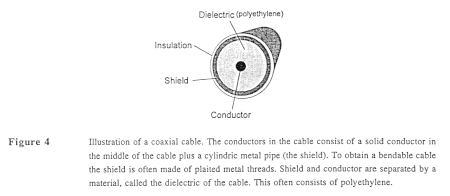
The shield of the coaxial cable (see FIGURE 4) is connected to
ground and therefore has the electric potential 0.0 V. The electromagnetic waves produced by
the step pulse generator are launched into the conductor of the coaxial cable with a voltage drop
of
0.225 V between conductor and shield.
The sampler is connected to the step pulse generator with a coaxial cable. When the step pulse
generator starts to transmit the electromagnetic waves they travel through the coaxial cable and
reach the sampler. Electromagnetic waves travel with an enormous speed. If the dielectric of the
coaxial cable is vacuum the waves will travel with the speed of light (light consists of
electromagnetic waves). If the dielectric is polyethylene, the waves travel with a speed equal to
66% of the speed of light. Thus the time interval between the transmission of the waves starts
and their detection by the sampler is very short. A sampler generally consists of two main
components:
When the electromagnetic waves launched from the step pulse generator are detected by the
sampler, the sampler starts to measure the voltage between the shield and the conductor at a
certain time interval, thereby obtaining a set of data consisting of voltage as a function of
time.
The oscilloscope shows the simultaneous measurements of time and voltage obtained with the
sampler on a Liquid Crystal Display (LCD). This produces a curve called a trace (FIGURE 2).
Obtaining information from the metallic cable tester
When the electromagnetic waves are launched into a cable that is connected to the metallic cable
tester any change in the electrical properties of the cable will cause a partly or total reflection of
the waves. The amplitude (voltage) of the reflection depends on the type of change. Changes in
the electrical properties of the cable cause changes in the impedance. Impedance is the total
resistance of a conductor to AC current and is measured in ohms. Most common coaxial cables
have an impedance of 50 ohms.
The reflected waves are superimposed with the waves transmitted from the metallic cable tester
and return to the metallic cable tester. Here the voltmeter in the sampler detects a change in
voltage between the conductor and shield, and the timing device in the sampler registers the time
interval between the start of the transmission of the waves and the detection of the reflection.
When two waves with the same frequency are superimposed the voltage amplitude of the
resulting wave depends on whether the waves are in phase or in counter phase.
Reflected waves are either in phase or in counter phase with the incoming waves, and the voltage
amplitude of the reflected waves are a function of the change in impedance which causes the
reflection. If electromagnetic waves meet an increase in impedance the reflected waves will be
in phase with the incoming waves. If electromagnetic waves meet a decrease in impedance the
reflected waves will be in counter phase with the incoming waves (Sorensen, 1990).
Consider a situation where an electromagnetic wave meets a change in impedance which causes
total reflection of the wave. This happens in two cases, (I) when the cable is open ended (the
impedance tens towards infinity and the wave is reflected in phase) and (ii) when conductor and
shield are short circuited (the impedance tends towards 0 and the wave is reflected in counter
phase). The voltage amplitude of the reflected wave is in both cases the same as the wave which
meets the change in impedance (the incoming wave). However the resulting voltage amplitude
of the wave when the incoming wave is superimposed with the reflected wave is totally different
in the two cases. In case (I) where the reflected wave is in phase with the incoming wave the
resulting voltage amplitude is twice the amplitude of the incoming wave. In case (ii) where the
reflected wave is in counter phase with the incoming wave the resulting amplitude is 0.
In conclusion if the sampler detects an increase in voltage there is an increase in impedance
somewhere along the cable that is tested and if the metallic cable tester detects a decrease in
voltage there is a decrease in impedance somewhere along the cable that is tested. From the
measured voltage it is possible to determine the change in impedance that caused the reflection.
The amplitude of the reflection can be calculated if the initial voltage step and the impedances on
both sides of the change in impedance are known:
where:
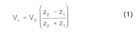
Vr: Amplitude of the reflection [V].
Rearranging EQUATION 1, z2 can be calculated if
Vr, V0,
and z1 are known.
V0: Amplitude of the voltage step launched into the cable [0.225 V].
z1: Impedance in the cable where the waves comes from [ohms].
z2: Impedance in the cable where the waves continue [ohms].
Because electromagnetic waves travel with an enormous speed the beginning of the waves is able to reach the end of a 900 m coaxial cable and get reflected back to the metallic cable tester within 10 µs if the dielectric is polyurethane. Tektronix has specified that the 1502B or C is able to test cables up to 500 m thereby securing that the beginning of the transmitted waves is able to reach the metallic cable tester within 10 µs which is the period the cable tester transmits the waves (see FIGURE 3). This is necessary because the whole principle behind the cable tester is based on that the reflected waves are superimposed with the transmitted. Otherwise the faults (changes in impedance) will not be detected. The pause lasting 50 µs secures that standing waves die before new waves are launched from the cable tester. From the measured time interval (read of the oscilloscope) it is possible to calculate the distance to the change in impedance if the velocity of propagation of electromagnetic waves in the cable is known.
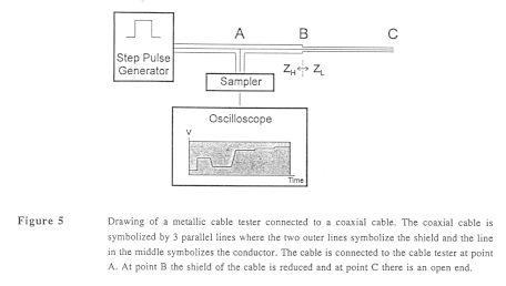
To clarify how the reflections of electromagnetic are superimposed (in phase or in counter phase) with the incoming waves and how the metallic cable tester obtains information from a cable we have created an example. This is shown in FIGURE 5.
At point A the cable tester is connected to a coaxial cable of the same type used internally in the cable tester (zH = 50 ohms). At point B the diameter of the shield is reduced. If only the diameter of the shield is reduced it lowers the impedance of the cable. This means that the impedance of the cable to the right of point B is less than 50 ohms (zL). At point C there is an open end. Because the end is held in air the impedance to the right of point C is tending towards infinity. As mentioned earlier the thereby induced changes in impedance at point B and C will cause reflections of electromagnetic waves.
What happens to the waves in the cable and how this is visualized on the oscilloscope is discussed in the following and is illustrated in FIGURES 6 and 7.
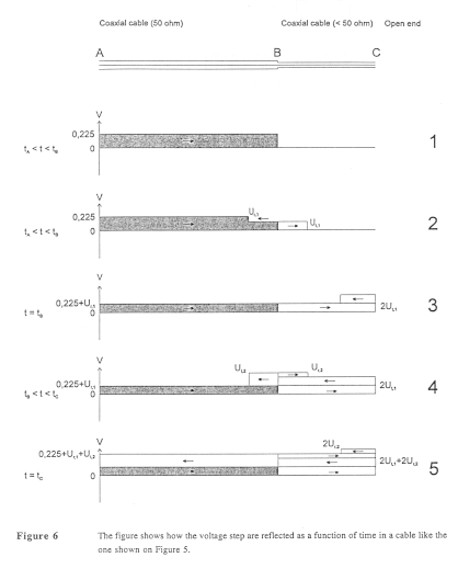
Time t = 0:
At t = 0 the step pulse generator starts to launch electromagnetic waves. Superimposed they
produce a voltage step of 0.225 V. At the same time the sampler starts to measure time and
voltage thereby obtaining a set of data (t,V). This is done with very small time intervals. The
measured values of (t,V) are transmitted to the oscilloscope where the measurements are shown
in a (t,V) system of coordinates. At time t = 0 the front of the voltage step has not yet reached
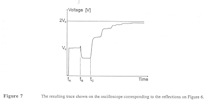
the sampler and therefore the sampler measures a voltage of 0.0 V (see FIGURE 7).
t = tA:
When the front of the voltage step reaches the sampler (at time t = tA), the sampler
measures a change in voltage between shield and conductor of 0.225 V. On the oscilloscope
this results in an instantaneously rise in voltage from 0.0 V to 0.225 V (see FIGURE 7). At the same time that the sampler detects the front of
the voltage step (t = tA) the front also enters the connected cable.
tA < t < tB (FIGURE 6.1):
The voltage step travels through the cable until it reaches point B. During this time the sampler
measures a voltage drop between shield and conductor of 0.225 V.
tA < t < tB at a later time (FIGURE
6.2):
At point B some of the voltage step is reflected back towards the cable tester (Ur,1)
and some is transmitted further on (Ut,1). Because the impedance of the cable to
the right of point B is smaller than to the left of point B the electromagnetic waves (remember
that the voltage step consists of electromagnetic waves) are reflected in counter phase with the
waves transmitted from the metallic cable tester. When a wave is superimposed with a wave in
counter phase it will result in a drop in amplitude in comparison with the original wave. This is
in agreement with EQUATION 1, where the amplitude of the
reflected
voltage
step (Ur,1) will be negative because z1 > z2. The
amplitude of the transmitted voltage step is equal to 0.225 V + Ur,1 =
Ut,1, because there always have to be the same voltage on both sides of a
discontinuity point (Sorensen, 1990).
t = tB (FIGURE 6.3):
The transmitted voltage step (Ut,1) continues to point C where it is totally reflected
in phase while the impedance on the right of point C tends toward infinity (an open end). Thus
the amplitude at point C becomes 1 Ut,1. At time t = tB the front of
the reflected voltage step (Ur,1) has reached the sampler, and the sampler detects a
drop in voltage between shield and conductor (see FIGURE
7).
tB < t < tC (FIGURE 6.4):
After a while the reflection of the transmitted voltage step (Ut,1) reaches back to
point B. Because the impedance is lowest where the voltage step comes from (~ z1
in EQUATION 1) the partly reflection (Ur,2) of the
electromagnetic waves toward point C is in phase. The transmitted voltage step
(Ut,2) towards the metallic cable tester is also in phase and equals Ut,1
+ Ur,2.
t = tC (FIGURE 6.5):
The reflected voltage step (Ur,2) reaches point C and is totally reflected in phase as
Ut,1. At t = tC the transmitted voltage step Ut,2 reaches
the sampler at point A. Because Ut,2 is in phase with the waves transmitted from
the cable tester the sampler registers a rise in voltage measured between conductor and shield.
From FIGURE 7 it can be seen that the time it takes the voltage
step to travel the distance from point B to C and back to point C is tC -
tB. This time interval is used in determination of the soil water content as will be
shown later. The total reflection of Ur,2 at point C will eventually reach point B
where some of its is transmitted towards point A and some is reflected back towards point C.
This continues periodically until the waves die and thus is responsible for the stair-shaped
voltage changes at t > tC (see FIGURE 7).
Measurements of soil-water content with TDR
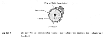
The velocity of propagation (v) of electromagnetic waves in a transmissionline is a function of the dielectrical materials between the conductors (see FIGURE 8).
Dielectric losses and relaxation phenomenons cause the retardation of the propagation of the waves (Heimovaara, 1993). This is expressed in the complex dielectric constant (K*). The connection between K* and the velocity of propagation of an electromagnetic wave is (Dalton et al., 1984):
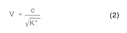
where:
In soil the complex dielectric constant can be described as (Topp et al., 1980):
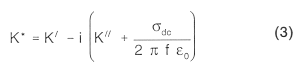
where:
If the electric loss in the soil is small then the imaginary part can be neglected (Topp et al., 1980) reducing EQUATION 3 to:
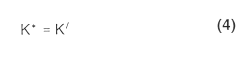
Over the frequency range of 1 MHZ to 1 GHz, the real part of the dielectric constant in soil does not appear to be strongly frequency dependent (Davis & Annan, 1977). The electromagnetic waves launched from the cable tester mainly consist of frequencies in this frequency range (Tektronix, 1987). A measurement of K' in a soil with low electric loss within the mentioned frequency range therefore in theory becomes only a function of the soil constituents. In practice, however, effects of electric loss and the different frequencies in the frequency range do influence measurements of K' to a small extent. Therefore a measured K' value is called the apparent dielectric constant and is denoted Ka.
As mentioned the TDR-measured dielectric constant in soil is approximately a function only of the soil constituents. The Ka values for the 3 main constituents are:
Water has a Ka value that clearly differs from the other main soil constituents. This
means that even small changes in the water content of the soil causes great changes in
Ka. A calibration between Ka and the soil-water content (![]() ) makes it possible to determine
) makes it possible to determine ![]() with TDR. Various
calibration functions are discussed by Jacobsen & Schjonning (1994, present
proceedings).
with TDR. Various
calibration functions are discussed by Jacobsen & Schjonning (1994, present
proceedings).
Determination of Ka in soil with TDR
The Ka value of a soil is determined with TDR by substituting the dielectric between conductor and shield with soil. Recall the example of reflections (FIGURE 5). Launching electromagnetic waves into this system (FIGURE 5) with soil as dielectric in the cable results in a trace equal to the one shown in FIGURE 7.
The time interval tC - tB is the time it takes for the electromagnetic waves to travel the distance from point B to point C and back to point B (equal to two times the length of the cable = 2 L). If the dielectric between point B and C in the cable is substituted with soil, the time interval tC - tB is a function of the water content in the soil. The relationship between Ka, tC - tB and L is:
Knowing the length of the transmission line which has soil as dielectric and measuring tC - tB from the TDR trace it is therefore possible to determine the Ka value of the soil with TDR.
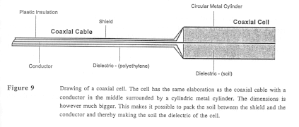
It is unpractical to substitute polyethylene with soil in a coaxial cable. Topp et al. (1980) therefore used a so-called coaxial cell in extension of the coaxial cable (FIGURE 9).
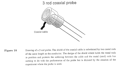
Use of the cell is feasible in some controlled laboratory measurements. However if there is some kind of water movement involved in the measurements the coaxial cells is useless because of its construction that only allows water movement parallel to the cell. Inserting a coaxial cell in soil can also be quite destructive. If low destruction of the soil is required and/or water movement is occurring so-called probes are used instead as an extension of the coaxial cable. There are a lot of different types of TDR probes and we will only show one called the three rod probe for examplification (see FIGURE 10).
The three rod probe is actually a simplification of the coaxial cell. Instead of using a cylindric metal tube as shield, the shield is substituted by two metal rods on each side of the conductor. The symmetric construction of the coaxial cell is retained, but the probe is less destructive and allows water movement to occur perpendicular to the probe rods. Practical use of probes and probe design is discussed by Thomsen (1994, present proceedings) and Petersen (1994, present proceedings).
This study was supported by the Danish Centre for Root Zone Processes under the Danish Environmental Research Programme.
Dalton, F. N., W. N. Herkelrath, D. S. Rawlins, & J. D. Rhoades. 1984. Time domain reflectometry: Simultaneous measurement of soil-water content and electrical conductivity with a single probe. Science (Washington) 224:989-990.
Davis, J. L. & A. P. Annan. 1977. Electromagnetic detection of soil moisture. Progress report 1. Can. J. Remote Sensing 3. 1:76-86.
Fellner-Feldegg, H. R. 1969. The measurement of dielectrics in the time domain. J. Phys. Chem. 73:616-623.
Heimovaara, T. J. 1993. Time domain reflectometry in soil science: Theoretical Backgrounds. Measurements and Models. Ph.D. dissertation. Universiteit van Amsterdam.
Jacobsen, O. H. & P. Schjonning. 1994. Comparison of TDR Calibration Functions for Soil Water Determination. Present proceedings.
Petersen, L. W. 1994. Sampling volume of TDR probes used for water content monitoring: Practical investigation. Present proceedings.
Sorensen, J. T. 1990. Overspændinger og transient beskyttelse. Laboratoriet for elektriske anlæg og hojspændingsteknik. Aalborg Universitet.
Tektronix. 1987. Tektronix metallic TDR's for cable testing -- Application note. Tektronix Inc. Beaverton, Oregon.
Thomsen, A. 1994. Manual and Automated TDR measurements. Present proceedings.
Topp, G. C., J. L. Davis, & A. P. Annan. 1980. Electromagnetic determination of soil water content: Measurements in coaxial transmission lines. Water Resour. Res. 16:574-582.
Last modified: 06-10-98