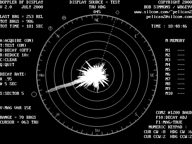
It has a ōsimulationö mode that allows the user to run the program with no input data.... you can download it and run it now... The COM port for the Doppler data can be either COM1 or COM2, at baud rates from 600 to 2400. ( my unit is 1200 ) It was deliberately written with an ōobsoleteö language, and features were kept to a minimum, ( monochrome ) so that it would be able to run on the greatest variety ( and oldest ) of computers. Anyway, itÆs free... Here is the download :
THE DISPLAY SCREEN
The visual presentation is oriented for ōrelative bearingsö, but you must keep the vehicle heading updated to ensure this remains true... The present DF bearing will always properly indicate ōrelative bearingö, even if the vehicle heading information is wrong. Vehicle heading is displayed at the 12 oÆclock position of the azimuth scale, and can be changed with the left / right arrows on the numeric keypad.

The various numeric readouts can be switched between magnetic and true
degrees, except for the numeric readout of the DF itself... that was kept ōrelativeö
so that the readings on this display could be directly compared with the reading
on the DF itself.
The last reported DF bearing is indicated with a large, empty circle ( the DF ōbugö ) located just outside the azimuth scale. An adjustable ōcursor lineö ( with numeric readout in bottom left screen ) can be moved to any position with the up/down arrows on the numeric keypad.... it is also indicated by a small empty circle ( cursor ōbugö ) outside the azimuth scale. Two more ōbugsö indicate magnetic and true North.
Ten memory ōslotsö are available to save a display and recall it later. Each can be ōtaggedö with a 7 character name or identifier, entered by the user on the keyboard. Keyboard entries are made ōwhen requiredö in the botton left corner of the display, which is ( otherwise ) kept empty, to minimize screen clutter.
THE FEATURES
The SECTOR function causes individual DF readings to be ōpaintedö in several adjacent bearings, as well as the ōproperö ( DF - reported ) bearing... For example, if the sector width is set for 10 degrees, a DF report at bearing 035 will be ōpaintedö at all bearings between 030 and 040. The sector size can be user - adjusted from 1 to 360 degrees. Default is 5 degrees.
This feature is provided because a single vector ōten readings longö is much more ( visually ) obvious than ten adjacent vectors ōone reading longö, even though they are ( probably ) of equal significance. Ten separate readings ( on adjacent bearings ) should probably be treated as a single bearing, since they probably originate from a single ( common ) radio source.
This feature is non-destructive and reversible... the source data is not changed. You can try various sector values to see the results, and then restore the original display by returning the sector size to its original value.
The DECAY function provides a means to slowly ōeraseö old bearings. This is achieved by multiplying ALL the displayed vectors by a specific fraction, ( between 0 and 1 ) at regular time intervals. The fraction value and time interval is user adjustable.... default is 0.95 fraction, at 5 second intervals. ( 1.0 fraction = no decay ) This method results in a ōstepwiseö approximation of an exponential decay.
If the decay function causes the longest vector to fall inside the largest ōrange ringö, the auto - ranging function will automatically ōdown - rangeö to a lower scale. As a result, the remaining display will still ōfillö the screen, but there will be fewer range rings. For learning purposes, try this : run the simulation until you get a display with 4 or 5 range rings, then turn off the ōacquireö function and turn on the ōdecayö function.
The decay function is destructive... results of each decay ōoperationö replace the original source data. If you want to restore the original display, save a copy of it in memory before turning DECAY on.
The REDUCE function is similar, but operates by SUBTRACTING a specific number from all vectors, instead of MULTIPLYING them by a specific fraction. As a result, the differences between the peaks and nulls is enhanced, and ( more importantly) between major and minor peaks, as well. This occurs because subtracting a specific number from all vectors will have a larger ōpercentageö effect on small vectors.
The number used for subtration is related to the range of the azimuth scale, and changes whenever the azimuth scale changes.... in all cases, it equals 10 percent of the scale currently displayed. For example, if the azimuth scale displays 4 range rings, the display scale is 50 readings. ( 4 rings + az scale = 5 rings @ 10 readings / ring ) Under these conditions, invoking the REDUCE function will cause all displayed vectors to be reduced by 5 readings.
The REDUCE function is destructive... results of each reduce ōoperationö replace the original source data. If you want to restore the original data, save a copy of it in memory before invoking REDUCE. Typically, the REDUCE function must be invoked several times in succession until the display yields the desired result.
There are also two ōsecretö features, not identified on the display screen.... they were not important enough to display them. Both of them involve the simulation mode of operation. One I call FOCUS, and the other I call REVEAL.
The FOCUS function determines the amount of ōrandomnessö of the simulated bearings. It is a number ranging from 0 to 1. A FOCUS value of 0 will cause a completely random display, and a FOCUS value of 1 will cause the random bearings to be very sharply ōfocusedö around the main ( simulated ) bearing.
The default value for FOCUS is 0.8. You can adjust FOCUS to smaller and smaller values ( = more random ) as you learn to ( effectively ) use the other features to identify signal direction. It can accept two digits of fraction information, ( example : 1.25 ) and can be invoked by hitting the ōFö key. The new value of FOCUS will not take effect until TEST has been turned off, and back on again. ( start another simulation )
The REVEAL function will ōrevealö the main bearing for the simulation, and can be used to confirm or refute your choice for the correct signal direction. It is invoked by hitting the ōFö key and entering ōRö or ōrö.... the correct bearing will briefly be displayed in the lower left corner. This value is expressed in RELATIVE degrees, so be sure to set the HEADING readout ( located at the 12 o'clock position of the azimuth scale ) to read "000" before you use the cursor to make your measurement of the "main lobe". Use the ( numeric keypad ) left and/or right arrow keys to do this.
REMARKS
Still, there are ( almost certainly ) significant differences between randomness caused by a computer program, and randomness caused by multipath and signal reflections... the true effectiveness of these tools can be proven ONLY with field tests...
Even in the simulation mode, there is plenty of room for ōcleverö use of the tools, either individually, or in combination.
I find the REDUCE function seems to work best with a large set of accumulated data, ( 1000 readings or more ) in which there is no clear ōmainö lobe. Invoking the REDUCE function many times in succession will enhance the main lobe, significantly. The larger the data set, the less chance there is to make a mistake... statistically, the main lobe MUST ( eventually ) have more bearings ( however slight ) than all the others. The REDUCE function will enhance this ōslightö difference, and make it obvious.
I find that the DECAY function can be used ( to some degree ) to measure the amount of ōrandomnessö of the signal bearing... this happens because the azimuth scale auto-ranges ōupö much more quickly if the signal tends to dwell around some specific bearing, ( within the window set by the value of SECTOR ) because the vector for that bearing will ōpump upö more quickly, as a result.
As the scale ōauto-ranges upö more and more, the spacing between adjacent rings becomes smaller and smaller, so it becomes harder and harder for a signal vector to ( consistantly ) remain in the area between the azimuth scale and the outermost ring...
Eventually, these two forces will achieve equilibrium, ( rate of vector growth and shrinking ring spacing ) and the display will tend to stabilize with a specific number of range rings...more rings implies greater DF bearing stability.
I also find that the SECTOR funcrtion is useful for revealing signal direction when used in a macroscopic way... setting the sector width to 30 degrees, 60 degrees, 90 degrees, or even higher will often reveal the general direction of a signal which appears completely random with a SECTOR value of only 5 or 10 degrees. In many cases, a general direction ( somewhere within 30 degrees of the real bearing ) is all that is really necessary to make a decision, since errors less than 90 degrees will ( eventually ) lead to success...
THE SIMULATIONS
The simulation runs at approximately the same speed as a ōrealö ( DF - generated ) display, which is approximately 7 to 8 DF readings per second. The acquisition speed is limited mostly by the math - intensive routines, such as the routines that generate the display vectors ( trig intensive ) and the SECTOR routines, especially if SECTOR is set to a large value.
... end of story...