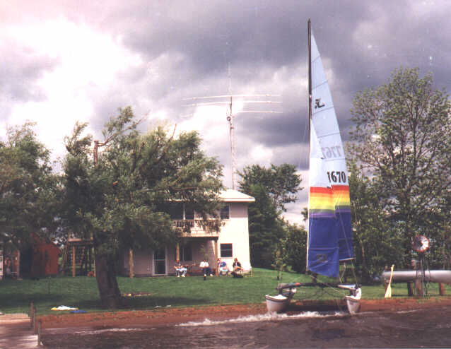
Bruce's cabin at Shell Lake, WI
BPSK and QRSS (Very slow speed CW) Signals
This part of the series includes a brief description of my receiving
equipment, some recordings of LowFER signals, and pictures of two stations
which have the most consistent DX signals at my location. My apologies
for leaving out LowFERs that have been heard here in past seasons, and
for not providing longer samples of the ones that are included. WAVE files
take up an awful lot of disk space, and I don't want to wear out whatever
welcome I may have on the qsl.net server. New photos may be added as they
become available.
My location is in a rural area, eight miles southeast of the town of
Aitkin in Central Minnesota, and about 100 miles north of Minneapolis.
The nearest neighbors are nearly a quarter of a mile away, and the electrical
line coming into the farm is buried for the 400-foot run between the house
and the road. With about 60 feet of separation between the shack and the
receiving loop, the noise generated by the receiver and its power supply
appears to be below the atmospheric noise level. Even in this location,
I have my best listening results late at night or in the early morning
hours when all the other electrical stuff in the house is shut down. To
the extent that it can be shut down, that is. It seems that almost everything
nowdays has a microprocessor in it that never sleeps. Examples are the
VCR, microwave oven, TV, and satellite receiver. I haven't taken a portable
receiver around the house to "sniff" out whether these things are generating
LF noise. Maybe it's best not to know.
Receiving equipment
My primary receiver is an ICOM IC-751A ham transceiver. The IC-751A
came with a 500 Hz CW filter in the second (9 MHz) IF as standard equipment.
Since I planned to use it for LowFER listening, I also bought the 250-Hz
filter for the third (455 kHz) IF. By using both filters at the same time
in combination with the passband tuning control, it is possible to slide
the response curve of one filter with respect to the other and vary the
effective bandwidth. With the settings I normally use to receive LowFERs
and NDBs, the filter bandwidth is approximately 100 Hz. I've found the
IC-751A to be an excellent receiver for LowFER listening. Like many other
radios, it apparently switches in an attenuator below 1.5 MHz. However,
unlike most radios, the attenuator is switched out again when you tune
below 500 kHz. Even so, I use a high-gain preamp in front of it for LowFER
listening, nearly always in combination with the 8-foot receiving loop
antenna described in Part 1 of this series.
In addition to the narrow IF bandwidth, I have tried various types of audio filters on the receiver's output. Many of the recordings in this article were made with a modified Timewave DSP-59+ audio filter. A description of the modifications is available in the Longwave web page file libraries. The modifications provide a tunable filter center frequency, and a mimimum bandwidth less than half of the bandwidth of the "stock" DSP-59+. Supposedly the minimum bandwidth of the unmodified filter was 25 Hz, but my measurements showed it to be closer to 36 Hz. The modified filter has a bandwidth of about 15 Hz when set to a center frequency of 400 Hz. Is all this filtering necessary? Maybe; maybe not. The typical human ear has an effective bandwidth of about 20 Hz at frequencies between 400 and 500 Hz. An experienced CW operator can pick out weak signals almost as well with a bandwidth of over 2 kHz as with a very narrow bandwidth. That is especially true in the presence of strong static crashes, which cause "ringing" in most narrowband filters. To my knowledge, the DX record for reception of a LowFER beacon was set in 1986, when Beacon "Z2" from San Simeon, CA was heard in Kauai, Hawaii. The receiver was a Realistic DX-200 without any narrow-band filters!
There are times when a very narrow audio bandwidth is useful. When you have a visitor in the shack who doesn't know (and probably doesn't care) how to pick out a weak CW signal in a broad wash of noise, you can switch in the audio filter and say "That signal". Chances are the visitor still won't recognize it, but will act impressed just to be polite. The other time when a narrow filter helps is when there is a strong carrier or other beacon very close to the desired signal. Although the human ear can detect very small changes in pitch, it is difficult to resolve two signals closer than about 50 Hz apart. For example, there is a very strong carrier at 189.0 kHz at my location (even when the Iceland LW broadcast station isn't coming in), and another weaker one at 189.080 khz. With only the 100-Hz IF filter to help me, I would not have been able to receive "NC" (formerly ZIA) when it was operating at 189.050 kHz. There are many other strong carriers within the LowFER band; some of them probably power-line carrier (PLC) signals, and others are just junk radiated by things like TV horizontal oscillators and switching power supplies. A narrow filter isn't always essential, but it normally doesn't hurt. That is, provided you're listening in the right place, which means that your receiver readout has to be accurate, as well as the information on the beacon you're looking for. It is also necessary to have a filter bandwidth that is wide enough to pass the "modulation" on the signal. Most LowFER beacons do not use keying speeds faster than 15 WPM, and I find that my narrowest audio filter setting does not degrade the signal except for a "softening" of the keying. One case where the filter bandwidth can be too narrow is when you are tuning around for stations that may not be listed, or listed incorrectly. With a listening time of 30 seconds at every 10-Hz frequency step, it would take over 9 hours to scan from 175 to 190 kHz! A filter that's too narrow can also degrade the copy when there are many strong static crashes. Even the best filters introduce some "ringing", which can completely obscure the desired signal if the filter gets hit by rapid static crashes. The majority of my listening for LowFER DX signals is done with the narrowest IF filter setting but without the audio filter.
The question sometimes comes up whether a narrow IF bandwidth is necessary at all if you have a good audio filter. If the receiver were "ideal" in the sense that it had "linear" mixers and infinite dynamic range at all stages, it would make no difference whether the filtering was done entirely in the IF or entirely at audio frequencies. However, a narrow IF filter will prevent the receiver from being overloaded and desensitized by strong nearby signals. The general rule in receiver design is to put the filtering as close to the antenna as possible to prevent overloading by signals outside the desired passband. It's also nice to be able to see a relatively weak LowFER signal actually move the S-meter. On all but the weakest detectable signals, I can almost copy the CW by watching the meter (if the static crashes aren't too bad) with the narrowest IF setting. But with a 500 Hz or wider IF filter, it takes a strong signal to show any variation from the background noise level.
These recordings are .WAV files saved in Microsoft ADPCM 8000 Hz, 4-bit monaural format. This a compromise between file size and the quality of the recordings, as well as their compatibility with various audio players. When playing these files with a browser like Netscape or Internet Explorer, another copy of the sound player is brought up every time you click on a link to a .WAV file. To keep from having a dozen copies of the application running at once, close the sound player manually before clicking on the next .WAV link. Another option is to click on the beacon link with the right mouse button and save the file to your disk, rather than playing it with the browser's built-in application.
There have been reports of incompatibility between the compressed .WAV
file formats on this page and the sound players in other computers. I have
been able to play them on two different computers using the standard "Sound
Recorder" applications in both Windows 3.1 and Windows 95 and the sound
player applets in Netscape 3.0 and Internet Explorer. But these .WAV files
will not play on another computer that I have, when I try to play
them in Netscape 2.0 or with the Windows 3.1 Sound Recorder. In my case,
the problem is not with the sound card, because they will play when
opened with either the Cool Edit or GoldWave shareware sound editors. If
you are unable to play the .WAV files on this page with your present software,
try downloading either the Cool Edit or GoldWave shareware. They are fun
programs to have on your computer anyway. Cool Edit includes a spectrogram
display, calibrated VU meter, an instantaneous frequency analysis feature
and a filter function, in addition to all the special effects and editing
capabilities. It also has a loop option which is very helpful when you
need to play the recording several times to pick the identifier out of
the noise. The latest versions of Cool Edit may be found at http://www.syntrillium.com/load.htm,
and both Cool Edit and GoldWave can be downloaded from http://sdc.wtm.tudelft.nl/sdc/tools.html
The obvious solution would be to use a more universally recognized
.WAV file format, like 8000 Hz, 8 bit, but that format requires double
the server space and download time.
I'll start with a recording of LEK made by Bill Bowers in Davenport, OK, a distance of about 750 miles. That's the best DX report to date on LEK in CW mode (Bill de Carle has copied LEK's BPSK signal in Quebec at about 925 miles). As you can hear, LEK wasn't exactly booming in. During three repetitions of the identifier, one is fairly clear (hey, it's all relative) but the others are almost obliterated by static crashes. Bill's receiving equipment does a tremendous job of smoothing the static crashes without ringing or ear-splitting pops -- the crashes just cause LEK to disappear momentarily.
The remainder of the recordings are of LowFER signals received here in central Minnesota. I have included only the beacons that I actually heard during the 1997-1998 winter season, and in the fall of 1998. Some of the recordings were made in previous seasons, although I believe they still represent the current format of the beacon identifier. Here they are in alphabetical order:
A3O Monroeville, PA, 806 miles. Not heard during
the 1997-1998 season but back again in the fall of '98.
ARK from Leslie, AR, 734 miles. Fairly consistent
here, although I don't believe the beacon is on the air during much of
the year.
BA in Lancaster, IL (near Mount Carmel), 623 miles.
Operated by Brice, W9PNE, BA was my first LowFER skywave QSO (and Brice's
IE beacon provided the only MedFER two-way contacts I've ever made).
BK from my son Bruce's cabin at Shell Lake, WI,
95 miles. BK's message format usually includes the wind speed and indoor/outdoor
temperatures after three repetitions of the identifier. From the parking
lot at his workplace in the Twin Cities, Bruce can make sure the pipes
aren't freezing in winter and check on windsurfing conditions in summer.
Bruce is using a novel LF antenna consisting of a grounded tower, with
a triband beam insulated from the mast to serve as the top hat for the
LowFER antenna. In the picture of the BK QTH below, the LF loading coil
is just visible at the top of the tower. When Bruce first put this antenna
into operation, the signal was down considerably from his old antenna.
However, with the help of a new loading coil and the onset of really cold
weather, BK seems to be as strong now as it ever was.
Bruce's cabin at Shell Lake, WI
BOB, Mahomet, IL, 504 miles. This is a cut
from Bob's special holiday message, recorded on 12/22/98. Bob is keeping
up the LowFER tradition of sending a special greeting during the holidays.
BRO from Duluth, MN, 70 miles. The newest of
a group of "local" LowFER beacons that I can hear any time of day. Bryce's
antenna is located very close to some large trees, and his signal improved
considerably with the arrival of cold weather.
GIR, New Eagle, PA, 810 miles. Heard a number
of times over the past few years; back again in the fall of 1998.
JDH, Bonaire, GA, 1095 miles. Until early 1998
when RED came through from Florida, the most distant LowFER beacon I've
copied on CW.
KRY from Chardon, OH, 712 miles. If I remember
correctly, the first LowFER skywave signal I ever heard. Joe sends his
complete QSL address, which took me at least a dozen passes of the message
to copy in its entirety the first time.
MEP, Paragould, AR, 734 miles. Same distance
from me as ARK, but in a different part of Arkansas.
NC from Stanfield, NC, 1029 miles. This one required
a very narrow filter and a listening period in the early morning hours
when the Iceland longwave broadcast station had started to fade. NC is
now operating on a new frequency that is further removed from the Iceland
carrier.
OK, Davenport, OK, 752 miles. Bill Bowers' OK
beacon is often readable here well into the daytime hours, sometimes even
during the summer. Bill manages to squeeze every last tenth of a dB out
of his antenna installations. The pictures below show his "OK-2" antenna
just after it was erected, and a closer view that gives a better look at
the top hat.
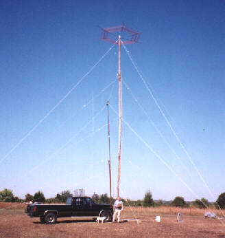
Bill Bowers and his OK-2 antenna
The antenna mast is made from PVC pipe wrapped with copper screen, and there are strips of copper screen plus multiple wires connecting the 10-foot radials in the top hat. Lots of top hat capacitance. Unfortunately, lots of wind loading too. At last report OK was transmitting from the old antenna after a severe wind storm folded the top hat on this one.
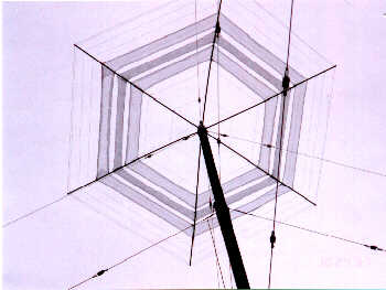
OK-2 top hat
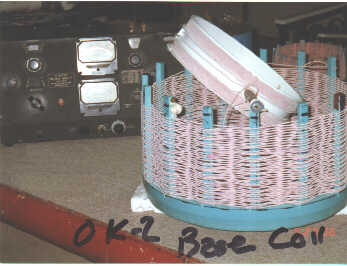
Besides having an excellent ground system, Bill uses very high Q loading coils that are basket wound with heavy Litz wire. The picture below shows the OK-2 base loading coil. A smaller rotating coil inside the large one forms a "variometer" configuration for fine tuning of the antenna system. If you're familiar with the Boonton Q meter in the background, it gives you a reference for the size of the loading coil. There is also a fixed loading coil with an inductance of 1.5 millihenries, mounted just below the top hat.
The photograph on Bill Cantrell's QSL card is a lot clearer than this
compressed image. If you look closely, you can see several of the extended
CB whip antennas that make up the 10-foot top hat radials.
X in Wheatland, WY, about 750 miles. This recording
was made in a previous season. So far this year the conditions haven't
been as favorable in Max's direction, although X is sometimes readable
during the early morning hours. I haven't been doing as much listening
as I used to, either.
YHO from Mason, OH, 785 miles, is another beacon
that returned in the fall of '98 after not being heard at my location for
a couple of years.
BPSK and QRSS (Very slow speed CW) Signals
There are several techniques for extending the range of LowFER beacons well beyond the distance at which they can be copied by ear. My article on "BPSK Basics" describes how to use the Coherent BPSK (C-BPSK) software developed by Bill de Carle, VE2IQ. This mode has been used successfully by a number of LowFERs and consistently outperforms CW for "real-time" operation -- that is, at speeds equivalent to 5 WPM and above. BPSK decoding software is free and may be downloaded from Bill's web site. Until recently, however, a special interface circuit called a Sigma Delta board was required between the receiver's audio output and the computer. Now Bill de Carle has developed a new version of the software called AFRICAM which uses a sound card input, so that just about anyone with a reasonably recent computer can receive C-BPSK signals. C-BPSK requires very good frequency accuracy at both the transmitting and receiving ends -- something under 1 Hz total error for good performance at the typical LowFER signalling rate of 10 baud (corresponding to MS100 in Bill de Carle's software).
Another way of pulling very weak signals out of the noise is called QRSS. The Q signal "QRS" means "send more slowly", and "QRSS" is the equivalent of saying "send really slowly". A common QRSS speed is 0.3 WPM, at which it takes 4 seconds to send a single Morse "dit" (plus another 4 seconds for the minimum silent interval following the dit). Not exactly life in the fast lane, but with the help of digital signal processing software, it is possible to take advantage of integration over time, and extract a signal that is buried deeply in the noise. The popularity of QRSS is due to the fact that it takes no special hardware at the sending end, and a number of freeware programs are available to aid in detection of the signal. To send QRSS, all you need is a memory keyer that can be slowed way down, or a computer program plus a simple keying interface to the transmitter. My article on "Using a PC as a Beacon Message Generator" describes a keying interface and contains software which can be slowed down to almost any speed. One note of caution when using my software at slow speeds -- Set up your identifier (and message, if desired) with a speed setting of 10 WPM or more and then slow down the speed. The keyboard scan is slowed down in the same proportion as the keying speed, so if you are running at something like 0.3 WPM and then press a command key to make any changes, the software will take a long, long time to respond!
Another important note: Older versions of the BCN.EXE file will hang up if you are using a fast computer and set the CW speed much below 1 WPM. If you don't have a version of BCN.EXE dated 11/27/00 or later, go to my article on "Using a PC as a Beacon Message Generator" and download the latest copy of BCN.ZIP. This fix has also been incorporated into the PCTX program described in my article on "A PC-Based Frequency Synthesizer.
Several good freeware spectrogram programs are available for displaying the slow CW on a screen. Probably the most popular is Spectran, which can be downloaded (along with a number of other interesting programs) from http://home.wanadoo.nl/nl9222/software.htm Other software links can be found on the LWCA web site. Hardware requirements differ for the various programs; Spectran probably needs at least a Pentium class computer and a compatible sound card. It works fine on one of my computers with a Creative Labs SoundBlaster, but not on another computer with a different brand of sound card. When the spectrogram is displayed with the proper time scale, decoding the identifier is a simple matter of reading the dots and dashes on the computer screen.
Bill de Carle has written another really neat piece of software that will capture the slow CW, compress it by an amount you specify, convert the output audio frequency to whatever you want, apply bandpass filtering if desired, and save the output to a WAVE file. For example, a 10-minute sample of a QRSS signal at 0.3 WPM can be compressed by a factor of 32 to yield about 20 seconds of audio at approximately 10 WPM. If there is an interfering carrier 10 Hz away from the QRSS signal, it will be 320 Hz away in the time-compressed WAVE file. Of course, if the receiver or transmitter frequency is off by 10 Hz, the output frequency will also be 320 Hz away from where you expect to hear it. Early versions of CRUNCH required a Sigma Delta interface board, but version 2.8 provides a sound card input option.
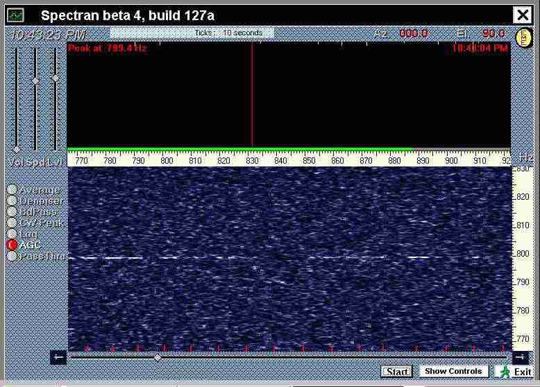
Here are two samples of QRSS signals "copied" with Spectran and with CRUNCH on the night of November 22, 2000 between 2130 and 2300 CST. Normally the spectrogram window in Spectran is dark blue, and the signals appear as white lines. For some reason, when I use the screen capture feature the dark blue background turns into multicolored clutter, but the signals still show up as white lines. In the Spectran screenshot shown below, you can see two repetitions of Bill Ashlock's "WA" identifier at 804 Hz. WA is located near Boston, about 1130 miles from the receiving location, and is the only LowFER I've copied that was using a loop antenna for transmitting.
After seeing the signal on Spectran, I ran Bill de Carle's CRUNCH program with a compression ratio of 32, output frequency of 450 Hz and output filter bandwidth of 50 Hz. The resulting WAVE file has been compressed into a 4-bit format and is included below as Wa.wav. Near the beginning of the 20-second recording (nearly 11 minutes in real time) the WA identifier appears twice, followed by a period of silence, then two slightly weaker identifiers near the end. Bill Ashlock uses a very novel transmitting setup with two crossed loops, and varies the loop phasing to shift the pattern in four steps. The silent period is apparently when the pattern null was in my direction, and I believe there was also some slow fading during the recording time.
Time-compressed recording of WA
After playing with the CRUNCH software, I went back to Spectran and ran it at a slower speed in an attempt to get an entire pattern rotation cycle. WA's signal was there, but had faded to the point where the dots and dashes were no longer distinctly readable; just broken lines at the 800 Hz frequency. Five minutes later, at about 2307 local time, there was almost nothing visible at 800 hz.
I had already heard JDH from Bonaire, GA in real-time CW this season. That was in the early hours of the morning when conditions were very quiet, and even then the signal was just barely readable. In the Spectran screenshot below, taken at about 9:30PM local time on November 22nd, there is one complete JDH identifier and the beginning of another one. The time-compressed JDH recording was made with a CRUNCH compression ratio of 32, which brings the CW speed from 0.4 WPM up to about 13 WPM.
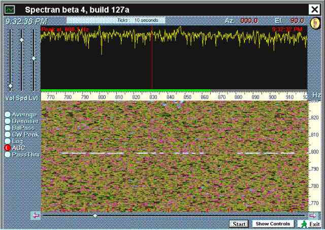
Time-compressed recording of JDH made on 11-22-00
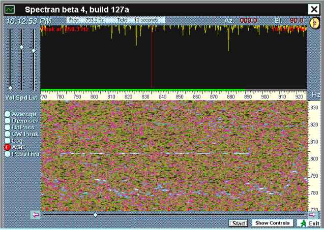
An interesting question is whether the audible output of CRUNCH or the visual readout of one of the spectrogram programs is better for detecting QRSS signals that are marginally readable. During the evening of 11-26-00, JDH was showing up as a faint trace on the Spectran display for an hour or more, but never got to the point where the identifier could be read distinctly from the screen. The screenshot below was taken at 10:43 PM and shows almost two complete identifier cycles although the Morse characters are not readable. By the way, the colors came out right this time -- wish I knew what I did that was different.
While one computer was capturing the Spectran data in the figure above, I ran CRUNCH on another computer to allow a direct comparison between these two QRSS receiving techniques. The resulting WAVE file is attached below. CRUNCH was set for an input frequency of 800 Hz, a time compression of 32, output frequency of 450 Hz and an output filter bandwidth of 50 Hz. I didn't do any "post processing" on the recording except to convert it to a more compressed (8k samples/sec, 4bit) format and increase the amplitude, which is a little weak in the WAVE files that I obtained using CRUNCH version 2.4. CRUNCH version 2.8 allows you to specify a gain number during the recording process, so that with a little experience you (and I) will be able to set the gain to a level that doesn't require tweaking later.
When played in continuous loop mode using Cool Edit or the Windows Media Player, I can pick out the JDH identifier fairly well after a couple of repetitions. Well enough to convince myself that I might be able to read the ID even if I didn't already know it. From this single comparison, it appears that the CRUNCH audio file offers a slight advantage over the visual display, which is in agreement with what I find on "real time" CW signals. However, there are a couple of important qualifications: Spectran was initially showing the JDH signal at 813 Hz, so I retuned my IC-706 receiver to 184.487 kHz (it uses LSB reception in the "normal" CW mode" to correct for the frequency error. If I hadn't done that, the CRUNCH audio output would have been shifted in frequency by over 400 Hz, well outside the filter passband. Actually the signal would have been shifted down (CRUNCH introduces another frequency inversion) and would have been below 50 Hz where it would be inaudible in my computer speakers even without any bandpass filtering. The other thing about the visual readout is the continuous indication -- you can glance at the screen from time to time and tell whether the signal is there. With CRUNCH, I have to take a stab in the dark by recording a WAVE file for several minutes and then play it back to see if a signal was present. To answer the question of which technique is better, it's nice to have both!