INTRODUCTION

An optical system is normally designed to give information about the object being viewed. Usually, the information appears in the form of an image. The amount and quality of information depends on whether the object is surrounded by a dark or light background (contrast), the size of the object (spatial frequency), and the quality of the optical system. The modulation transfer function (MTF) of an optical system is a measure of the system’s imaging capabilities and will largely determine the amount of fine detail that will be observed in the image. This module examines and explains in some detail the concept and utility of the modulation transfer function, particularly as it applies to resolution.

MODULE PREREQUISITES

The student should have completed Module 1-4, "Properties of Light"; Module 1-8, "Temporal Characteristics of Lasers"; Modules 2-8 through 2-11 of Course 2, "Geometrical Optics"; Module 6-1, "Optical Tables and Benches"; Module 6-8, "Lenses"; Module 7-8, "Mechanical and Bleachable Dye Methods"; and Module 9-6, "Power Supply and Calibration of a Photomultiplier." The student should also have a basic knowledge of algebra and geometrical and wave optics, and be able to operate a helium-neon laser, photomultiplier, and electrometer.

Upon completion of this module, the student should be able to:

1. Explain how the modulation transfer function of an optical system determines the quality of the optical system.

2. Explain the difference between the square-wave and the sine-wave MTF.

3. Calculate the MTF of an optical system, given the MTFs of the individual components.

4. Set up the equipment and measure the square-wave MTF of two lenses.

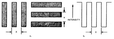
Historically, the earliest measure of performance for an optical component or instrument was resolving power. Resolving power of an optical system refers to the ability to separate two closely spaced objects in the image generated by the optical system. To test the quality of an optical system, it is common to test it with line patterns. The resolving power is commonly expressed in terms of a spatial frequency (i.e., lines/mm or line pairs/mm).

A type of object frequently used to test the performance of an optical system consists of a series of alternating light and dark bars of equal width with sharp boundaries, as indicated in Figure 1a.

If the pattern of the bars is repeated in X millimeters (1 period), then the pattern has a frequency of 1/X lines per millimeter (lines/mm). A plot of the intensity of the light transmitted by the bar target is shown in Figure 1b. When an image is formed by an optical system, each point is imaged as a blurred spot due to aberrations, diffraction, scattering, and absorption.

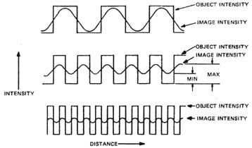
The usual procedure is to photograph such a test chart and then pick out the finest pattern in which individual lines can be identified. The reciprocal of the width of a line-plus adjacent-space is called the limiting resolving power of the system. As an example, the test chart shown in Figure 2 has been imaged by a 250 mm lens. This image is shown in Figure 3.

As the bar becomes smaller, it becomes more difficult to clearly identify the individual lines. For purposes of calculation, assume that the finest pattern which is discernible is group 1 element 1. The limiting resolving power of the optical system, which in this case includes the 250 mm lens and the photographic film, can be determined by measuring the period of the bar pattern in group 1 element 1 in the test target shown in Figure 2. The period is 0.5 mm. Thus, the limiting resolution for this hypothetical case is 2 lines/mm. The reason the lines are more difficult to see as the pattern becomes smaller is that the apparent change in intensity between the dark and white regions is decreasing as one approaches the limiting resolution of the system. The intensity pattern for several spatial frequencies is shown in Figure 4. (The spatial frequencies vary from low on the top curve to high on the bottom curve.)

The difference in intensity between the dark and white regions is the same for all frequencies at the object. But notice how it decreases in the image as the spatial frequency increases. The dark regions become lighter and the white regions darker, i.e., the contrast decreases. Also notice how the sharp discontinuities in the object have been rounded off in the image. When the contrast in the image is smaller than the system (e.g., the eye, film, or photodetector) can detect, the pattern can no longer be resolved.

The contrast C is defined in terms of intensity I, as given by Equation 1.

If the background is perfectly black, I_min = 0, then—

which is the highest contrast possible. If the bars and the intervals are mere shades of gray, the contrast decreases correspondingly. Least contrast will result if I_max = I_min, in which case C = 0. Thus, contrast may vary between zero and one. The human eye requires approximately 5% contrast to resolve an image.

Equation 1 is used to solve a problem in Example A.

Example A: Calculation of the Contrast
Given:	An intensity pattern such as the one shown in Figure 4 has a maximum intensity Imax = 0.85 and a minimum intensity Imin = 0.35.
Find:	The contrast of the intensity pattern.
	C =	(Equation 1)
Solution:	C = = C = 0.417

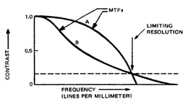
To evaluate an optical system, more information than the limiting resolution is required. To determine how much contrast can be transferred from the object to the image at all spatial frequencies, the modulation transfer function (MTF) is needed. The MTF is the ratio of the modulation in the image to that in the object as a function of spatial frequency. Thus, if one plots the contrast (image-to-object) as a function of spatial frequency, one obtains a curve (the MTF) for the particular optical component or system. Two such curves for two different imaging systems are shown in Figure 5. Notice that both systems have the same limiting resolution frequency. However, the system represented by A will produce a superior image because the greater modulation at lower frequencies will produce crisper, more contrasting images. Unfortunately, the type of choice that one is usually faced with in choosing a system is not as clear as that implied by the curves in Figure 5.

Consider the two systems shown in Figure 6, where one system shows limiting resolution (B) and the other shows high contrast at low spatial frequencies (A). In situations of this kind, the decision must be based on the relative importance of contrast versus resolution in the specifically intended function of the system.

The preceding discussion has been based on square-wave intensity patterns and the square-wave MTFs. However, if the object pattern is in the form of a sine wave, the intensity distribution in the image is also described by a sine wave. If the MTF is not indicated as square-wave MTF, it is generally assumed to be a sine-wave MTF.

Sine-wave targets are quite difficult to obtain, so generally it is easier to measure the square-wave MTF and then convert the square-wave MTF to the sine-wave MTF mathematically. There are systems that measure the sine-wave MTF of systems, but they are very costly compared to those capable of measuring square-wave MTFs. However, the square-wave MTF can be converted to the sine-wave MTF using the following equation:

Equation 3

MTF (f1) sine wave =

For example, if the square-wave MTF for a system is:

then—

at a frequency of 10 lines/mm. In this manner, the entire sine-wave MTF can be calculated.

Example B: Calculation of Bk Factor
Given:	Bk = if t = M; Bk = 0 if t < M.
Find:	Bk for k = 9 and k = 11.
Solution:	For k = 9, the number of different prime factors is one. The prime factor is 3.3. Thus, t = 1 and M = 2. Since t < M, Bk = 0. For k = 11, the prime factor is 11. Thus, t = 1 and M = 1. Since t = M, Bk = = –1 (–1)5 Bk = 1

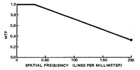
Figure 7 shows the square-wave response of an optical system and its sine-wave equivalent. A plot of MTF against frequency is an almost universally applicable measure of the performance of an image forming system, and can be applied not only to lenses but to films, image tubes, the eye, atmospheric propagation, and even to complete systems.

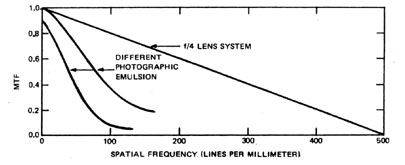
One particular advantage of the sine-wave MTF is that it can be cascaded by simply multiplying the sine-wave MTFs of two or more elements at each frequency of interest to obtain the MTF of the combination. For example, if a camera lens system with a sine-wave MTF of 0.4 at 30 lines/mm is used with film having a sine-wave MTF of 0.8 at this same frequency, the combination will have a sine-wave MTF of 0.4 ´ 0.8 = 0.32. If the object photographed with this camera has a contrast of 0.2, then the image will have a contrast of 0.32 ´ 0.2 = 0.064. However, note that the MTF of a system does not equal the product of the MTFs of the individual components if the components are not directly connected; that is, the lenses are not separated by diffusers. Aberrations of one component may compensate for the aberrations in other components in a system of lenses and, thus, produce an image quality which is superior to that of either component. Any "corrected" optical system illustrates this point.

Figure 8 shows the MTF for a correctly focused f/4 lens system free of aberrations, transmitting quasimonochromatic light of a mean wavelength l = 500 nm. The MTFs of two typical photographic emulsions are also shown.

Before beginning, familiarize yourself with and heed all appropriate safety rules concerning the use of laser systems. Avoid the hazards of high-voltage electrical systems. The following tasks will be performed:

1. Set up the equipment necessary to measure the square-wave MTF of lenses.

2. Measure the square-wave MTF of the poor-quality lens.

3. Measure the square-wave MTF of the poor-quality lens when the diameter of the lens is half that used in Task 2.

4. Measure the square-wave MTF of the high-quality lens.

The experimental arrangement as shown in Figure 9 should first be constructed. To minimize vibrations, it is recommended that the entire experimental apparatus be mounted on an isolation table.

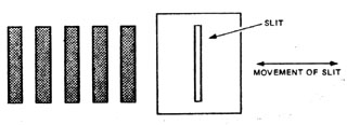
The expanded helium-neon laser beam impinges on a diffusing glass to eliminate the coherence of the laser beam and fully fill the test lens aperture. The spatial frequency target is mounted just behind the diffusing glass in a mount so that various spatial frequency targets can be placed in identical positions with the bars oriented vertically. The distance between the target and the lens to be tested should be approximately twice the focal length of the lens. A 632.8 nm filter should be mounted in a light-tight manner directly in front of the photometer to eliminate spurious room light from getting into the detector. This eliminates the necessity of performing the experiment in a darkened room. The one-micron slit is placed directly in front of the 632.8 nm filter, absolutely parallel to the bars of the spatial target, and the entire assembly (slit, filter, and detector) is mounted on the translator so that the slit can be moved across the image of the spatial target, as shown in Figure 10. This total assembly should be mounted perpendicular to the optical axis of the laser-lens-target system.

Move the translator with the mounted detector, filter, and slit so the image of the spatial target falls exactly on the slit. This adjustment is very critical because the resultant MTF will be considerably less if the spatial target is not focused properly on the slit, thus giving a misleading result.

The apparatus is now ready to measure the MTF of the lens. With the 0.25 line/mm spatial target in place, adjust the translator for a minimum reading (R₁) and record. Next, adjust the translator for a maximum reading (R₂) and record. From these two readings, the contrast of the image is calculated with the aid of Equation 5.

The C_object is equal to one because the bars are perfectly black. Thus,

To measure the square-wave MTFs at other frequencies, remove the 0.25 line/mm spatial target and replace it with the other spatial targets, and repeat the measurements. It should not be necessary to refocus the target onto the slit if care is taken to replace the spatial targets in the holder in identical orientation. In fact, at higher spatial frequencies (100 lines/mm or higher), it is impossible to see the bars without a microscope. Therefore, refocusing the lens is very difficult.

To perform Task 3, mount an iris directly in front of the lens and adjust the diameter so that it is half the size of the lens diameter. Now measure the square-wave MTF of the lens. Do you notice any difference in the square-wave MTFs of the masked and unmasked lens? What led to this result? Is it reasonable?

In Task 4, remove the iris and replace the poor lens A with the high-quality lens B. Place the 0.25 line/mm spatial frequency target in the holder. Move the translator with attached equipment until a sharp image is on the slit. Repeat the measurements as before to obtain the square-wave MTF.

Now by comparing the square-wave MTFs, the lens that would be best for a particular situation can be chosen. If this lens is going to be used in an optical system, the square-wave MTF of the lens has to be converted to a sine-wave MTF before the system MTF can be calculated.

Calculate the corresponding sine-wave MTF.