[
 Producing wound components]
[A guide to the terminology used in the science of magnetism]
[ Power loss in wound components]
[The force produced by a magnetic field]
[ Faraday's law]
Producing wound components]
[A guide to the terminology used in the science of magnetism]
[ Power loss in wound components]
[The force produced by a magnetic field]
[ Faraday's law]
Browser requirements: IE5 is the only one that seems to work at the moment. About fonts: if the character in brackets here [ × ] does not look like a multiplication sign then try setting your browser to use the Unicode character set (view:character set menu on Netscape 4). Also this character [ Φ ] is the Greek letter 'phi' in modern browsers.
See also ...
[
Producing wound components]
[A guide to the terminology used in the science of magnetism]
[ Power loss in wound components]
[The force produced by a magnetic field]
[ Faraday's law]
[Top of page]
Do you need an air coil?
What are the advantages of an air core coil?
You may be using an air cored coil not because you require a circuit element with a specific inductance per se but because your coil is used as a proximity sensor, loop antenna, induction heater, Tesla coil, electromagnet or deflection yoke etc. Then an external field may be what you want.
[Top of page]
The single layer coil
A single layer coil has two advantages. Firstly, like all air core coils,
it is free from 'iron losses' and the non-linearity mentioned above. Secondly, single layer coils have
the additional advantage of low self-capacitance and thus high self-resonant frequency. These coils are mostly used
above about 3 Mhz.
 In the simple case of
a single layer solenoidal coil the inductance may be estimated as follows
(Wheeler) -
In the simple case of
a single layer solenoidal coil the inductance may be estimated as follows
(Wheeler) -
  L = N2r2 / (228r + 254l)   microhenrys

       where  L is inductance in microhenrys
              r is the coil radius in millimetres
              l is the coil length in millimetres (>0.8r)
              N is the number of turns
This formula applies at 'low' frequencies. At frequencies high enough for skin effect to occur a correction of up to about -2% is made.
To construct a self-supporting air cored coil take a length of plain 1 millimetre diameter copper wire and hold one end in a bench vice. Take the other end in a pair of pliers and pull until the wire has stretched slightly - this will straighten it. Using a 5 millimetre diameter drill bit wrap the wire around it until enough turns have been applied. Using 'long nosed' pliers bend the ends of the coil to get them into a radial position.
Small reductions in the inductance obtained can be achieved by pulling the turns apart slightly. This will also reduce self-resonance. Other combinations of wire and coil diameter may be tried but best results are usually obtained when the length of the coil is the same as its diameter.
This property also leads to a disadvantage of the air cored coil: microphony. If you need good frequency stability in the presence of vibration then wind the coil on a support made from a suitable plastic or ceramic former.
[Top of page]
The multi layer coil
Figure 1 below shows a multi layer air cored coil wound on a circular coil
former or bobbin. (If the image is broken or scrumbulated then you need an
updated browser).
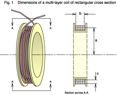
This type of winding is very common because it's simple to construct with a winding machine and a mandrel. We'll consider it in some detail. The first question is this: if you have a fixed length of wire then what dimensions of the winding give the greatest inductance? Put another way, what is the most efficient shape?
The ratio of the winding depth to length, which is c/b, needs to be close to unity; so the winding should have a square cross section. This makes sense because only with the square is the average distance between turns at a minimum (a circular cross section would be even better, but that is hard to construct). Keeping the turns close together maintains a high level of magnetic coupling ('flux linkages') between them, and so the general rule that the inductance of a coil increases with the square of the number of turns is maintained.
OK, now what about the mean radius of the turns: dimension a ?
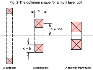
In the Fig. 2 above you see three coils in cross section. Each uses the same length of wire but the diameter of the coil varies. The inductance of any one turn is linearly proportional to its diameter; so you want a large diameter to get the most inductance. Also you need all turns in the winding to be as close as possible to all the others. The coil on the left fulfills these requirements, but it has a problem because, in making the diameter large, you don't have sufficient wire to give it many turns. Since the inductance of the winding as a whole varies as the square of the number of turns the left hand coil won't have high L.
The coil on the right does have a high number of turns, but it isn't optimum for two reasons. The diameter of each turn is small (particularly those near the centre of the coil) which leads to a low inductance per turn. Worse, the distance between turns separated by the diagonals of the winding cross section is large. This leads to weak coupling between them (lower flux linkage) and a failure of the N2 relationship with coil inductance.
Can you anticipate a punch line? Brooks, who wrote a paper in 1931, calculated that the ideal value for the mean radius is very close to 3c/2. We call a coil having these dimensions a Brooks coil. It's worth emphasising that the Brooks ratio is not critical. You can have a coil which deviates from it quite significantly before L falls off very much. Also, you may have other considerations than the inductance alone.
If we let S1 = (c/2a)2 then the inductance of any of our three coils can be approximated by
L = 4×10⁻⁷where a is the mean radius of the winding in metres.a N2((0.5+S1/12)ln(8/S1) -0.84834+0.2041S1) henrys
Example: If the mean radius is 2.4 cm, the width is 9mm and N is 350 then L = 6.977 mH.
If we have a proper Brooks coil then the formula above boils down to
L = 1.6994×10⁻⁶aN2 henrysExample: If the mean radius is 2.4 cm and N is 350 then L = 4.996 mH.
[Top of page]
Flux density in an air coil
[Top of page]
When the density is important
Sometimes the purpose of an air coil is not to possess inductance but to
create a region of space having a definite magnetic flux density. A well
known example of this is the deflection coils placed around a cathode ray tube
where the direction of the electron beam is controlled by the current driven
through the coils. Outlined below are methods by which you can relate
the strength of the field to the coil current. When you know the field
at all points around a coil then you can also find its inductance.
The Biot-Savart equation
 An important result of the work carried out by André Ampère
is the equation which is refered to as the Biot-Savart. This gives the
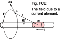
field at any point surrounding a current element. Such an element
should have negligible length and diameter (see figure FCE).
An important result of the work carried out by André Ampère
is the equation which is refered to as the Biot-Savart. This gives the
field at any point surrounding a current element. Such an element
should have negligible length and diameter (see figure FCE).
dB = μ0 I ds sinθ / (4π r2) teslasThis shows that the magnitude of the field falls with the square of the distance, r, from the current element and also with the sine of the angle subtended to the current direction, θ. The direction of the magnetic field is at a right angle to the current direction and also at a right angle to the line r. The 'sense' of the field vector is right handed or clockwise looking along the direction of current flow.
At any point along the circular field line labeled F in figure FCE a tangent to it has a direction fulfilling the requirements just given. Imagine a set of such lines surrounding the current element, spaced in accordance with the expression for dB.
You might complain that the Biot-Savart equation doesn't seem to be buying us
very much: an isolated current element is an imposibility in practice and real
coils use wires which may be very thick. What saves the day in the case of air
coils is the priciple of superposition. Without a ferromagnetic core to spoil
the linearity of the system we can simply divide the actual current flow up
into any number of smaller regions and then sum, or integrate, the individual
fields to obtain the total flux density.
Biot-Savart solves a current loop
Let's apply Biot-Savart to a single turn circular loop
and derive a formula for the flux density at
any point along the axis. We'll assume that the diameter of the wire is
negligible in comparison with the diameter of the loop - in the terminology
this is known as a current filament.
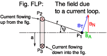 In figure FLP we see the loop in cross section and we want
the flux density at the point P1 on the loop axis at a distance
r from the conductor. We start by considering the contribution to the
field made by a current element at P2.
The figure shows a P1 which happens to be quite far from the loop.
ψ is rather small and the field vector (BT,
shown in blue) is swinging up towards a normal to the axis of the coil.
You can resolve BT into two components: BN, shown in red
and BA, shown in green. We can disregard the normal component,
BN, because of the symmetry of the loop: it is going to be cancelled
by the field generated by the current element on the opposite side of the loop
at P3. We are left with just the axial component (that we need to
find): BA. Its magnitude will be
In figure FLP we see the loop in cross section and we want
the flux density at the point P1 on the loop axis at a distance
r from the conductor. We start by considering the contribution to the
field made by a current element at P2.
The figure shows a P1 which happens to be quite far from the loop.
ψ is rather small and the field vector (BT,
shown in blue) is swinging up towards a normal to the axis of the coil.
You can resolve BT into two components: BN, shown in red
and BA, shown in green. We can disregard the normal component,
BN, because of the symmetry of the loop: it is going to be cancelled
by the field generated by the current element on the opposite side of the loop
at P3. We are left with just the axial component (that we need to
find): BA. Its magnitude will be
BA = BT sinψThe Biot-Savart equation gives us dBT so we can combine the two to get
dBA = μ0 I ds sinθ sinψ / (4π r2)Clearly, any line (such as r) which joins P1 to the conductor will intersect the direction of current flow at a right angle. This means that sin(θ) in the Biot-Savart equation will be 1.0. At points off axis this won't always be the case and the maths gets harder.
dBA = μ0 I ds sinψ / (4π r2)Now, all we have here is the field due to the single current element at P2, but we need the total field due to all the elements around the loop. Fortunately, because of the symmetry all the elements contribute the same as P2, so to do the 'integration' we need only multiply by the path length around the loop: 2πa -
BA = a μ0 I sinψ / (2 r2)Substituting r = a / sinψ -
BA = a μ0 I sinψ / (2 (a / sinψ)2)so
BA = μ0 I sin3ψ / (2a)And if the coil is multi-turn then superposition again gives
| BA = μ0 Fm sin3ψ / (2a) teslas | Equation FMC |
| Symbol | Purpose |
|---|---|
| N | The total number of turns in the solenoid |
| b | The length of the solenoid (metres) |
| a | The radius of the solenoid (metres) |
| P1 | The point on the axis at which we need to find the flux density |
| z | An arbitrary distance along the axis from P1 |
| ψ | The angle subtended at P1 by the axis and a point at the top of the winding at z |
| ψ1 | The angle subtended at P1 by the axis and the top of the winding at the left hand end |
| ψ2 | Ditto for the RH end |
| I | The solenoid current (amps)
|
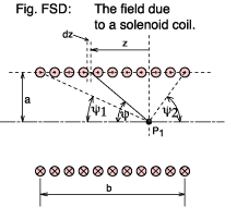
First we have to make a simplification because the flux lines will not run perfectly true along the axis but will spiral slightly around it (reflecting the helical nature of the coil itself). This effect becomes less if the turns are spaced more closely. In fact this leads on to the concept of a current sheet. If we kept the dimensions of the solenoid the same but used, say, three times the number of turns and at the same time reduced the current to one third then the overall magneto motive force is the same and so the field produced will be much as before.
In the limit we no longer worry about the total number of individual turns and the coil current. Mentally replace them with a thin walled copper tube carrying a total current N × I amps flowing around its circumference and distributed evenly along its length. Don't ask how the current gets there; this is pure hypothesis :-) . Now we can talk of an mmf per unit length of the tube, Fl -
| Fl = I × N / b amps per metre | Equation MLT |
Fm = Fl dzSubstituting this into eqn. FMC
dB = μ0 Fl dz sin3ψ / (2a)This represents the contribution to the flux density at P1 due to a current loop whose perimeter subtends an angle ψ with the axis at P1. From the geometry
z = a / tanψSubstituting this into the equation for dB givesdz/dψ = -a cosec2ψ
dz = -a dψ cosec2ψ
dB = μ0 Fl (-a dψ cosec2ψ) sin3ψ / (2a)For the part of the tube between P1 and the left hand end ψ will take values between π/2 and ψ1dB = -(μ0 Fl / 2) sinψ dψ
B = -(μ0 Fl / 2) ∫ sinψ dψ
B = -(μ0 Fl / 2) π/2∫ψ1 sinψ dψThe part of the tube to the right of P1 will superpose an additional flux at at P1 -B = (μ0 Fl / 2) [cosψ]π/2ψ1
B = (μ0 Fl / 2) cosψ1
| B = (μ0 Fl / 2) (cosψ1 + cosψ2) teslas | Equation FDS |
B = μ0 Fl teslas
[Top of page]